The RTflow Help is organized into the following main parts:
| Term | Description |
|---|---|
| Active file | The file that is in view in the tab area, if any. A file is made active by clicking its tab. |
| Block | A building block for schematics, for example an input port, an adder or a user block. When there is no risk for confusion, "block" will also refer to a block instance. |
| Block instance | An instance of a block in a schematic. For example, there may be several instances of the block Add in a schematic. |
| Blocks tree | A tree containing all available blocks for use in the schematic editor, available under the Blocks tab in the tree view in the left part of the main window. |
| Causality loop | A set of blocks that are connected in a loop without any delay (Pre) block. Causality loops are illegal in RTflow and will generate a compiler error. |
| Command | A function in RTflow that can be invoked by the user through a menu, a toolbar button or a keyboard shortcut. |
| Connection | A connection between port instances in a schematic. A connection specifies that all input and output ports that the connection is attached to have the same value at each cycle. |
| Constant | An input whose value is a constant value specified at design/compile time for each instance. In a schematic, the user specifies the value in editable fields directly in the block, or in the block instance properties window. For example, the primitive block Gain has a constant specifying the amount of gain. |
| Cycle | A discrete time step, also called execution cycle or instant. During the execution of a model, all signals are updated exactly once per cycle. |
| Element | See Schematic element. |
| Equation | A subnode or the usage of a primitive function within a node. Each block instance corresponds to an equation with the same name. |
| Execution cycle | See cycle. |
| Frame | An add-on of graphics to schematics, typically used to enhance the appearance of a printed schematic. |
| Graph area | The right part of the simulator view, showing graph plots of signals values over time. |
| Instance | See Block instance. |
| Joint view | A display mode of the graph area, where several graphs are displayed in one common coordinate system. |
| Main window | The main application window that opens when RTflow starts, and that contains the menu, the tree view, the tab area and the message view. |
| Node | The function of a non-primitive block. Each schematic corresponds to a node with the same name. |
| Primitive block | A block whose function is hard-coded in RTflow, as opposed to a standard block or a user block, whose functions are defined in schematics or other source files. The Add block is an example of a primitive block. |
| Project | A set of source files and settings for simulation, code generation et c for these source files. |
| Project tree | A visualization of the set of source file, available under the Project tab in the tree view in the left part of the main window. |
| Port | An input or output of a block or a schematic. When there is no risk for confusion, "port" will also refer to port instance. |
| Port instance | A port on a block instance in a schematic, symbolized by a small line on the edge of the block instance. Port instances are the endpoints of connections. |
| Sample time | The real time duration of one execution cycle. |
| Schematic | A sheet containing blocks, connections and other graphical elements that define the behavior of a system or a sub-component of the system. |
| Schematic element | A block instance or a connection. |
| Signal | The bearer of a value that changes with time during simulation or execution. This is the same as a variable in many other programming languages. Each connection in a schematic corresponds to a signal with the same name. |
| Signal area | The left part of the simulator view, showing signal names, values and other signal attributes in a table. |
| Simulator view | The view that opens under the Simulator tab when the simulator is started. It consists of the signal area, the graph area and a toolbar. |
| Source file | A file that is part of the project and that can be compiled. In the current version of RTflow, schematic files are the only source files. |
| Split view | A display mode of the graph area, where each graph is displayed in an individual row. |
| Subnode | The instance of a node within another node. Each non-primitive block instance corresponds to a subnode with the same name. |
| Standard block | A block whose function is defined in a source file that is delivered with RTflow, for example the Integral block. |
| Symbol | The graphical representation of a block. |
| Tab area | The main area of the application window where the source file editors and the simulator open. |
| Tree view | The left part of the main window, showing either the project tree or the blocks tree. |
| User block | A block whose function is defined in a source file not delivered with RTflow. Typically these blocks have been compiled from source files in the user's project. |
The purpose of the tutorials is to present the different aspects of RTflow and guide through the most common functions. After completing the three tutorials, which should take no more than 15-20 minutes each, you should be fully prepared to start making your own models with help from the subsequent reference sections.
The three tutorials are:
This tutorial presents the basic functions in RTflow by explaining how to design a simple counter, simulate it and finally generate C++ and VHDL code from it. The complete files for the design can be found in the /Examples/Counter folder under the application folder; however, this tutorial will explain how to create the same files so they are not needed for the exercise.
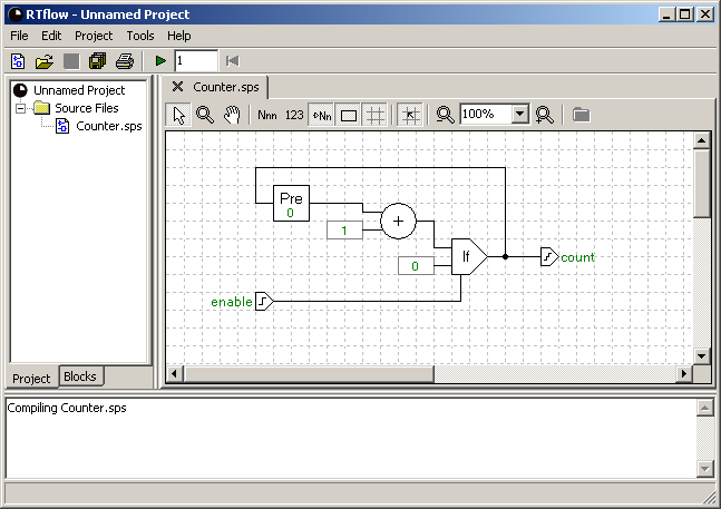
The functionality of the counter is very simple: it has one boolean input signal enable and one integer valued output signal count. When enable is 0, count is 0. When enable is 1, count is the number of cycles that enable has been 1. The schematic for the counter, which will be created during this tutorial, is shown below.
The counter illustrates two basic properties of RTflow's execution model:
Mathematically, the counter can be expressed as a function from sequences of boolean numbers to sequences of integers as follows:
	count[0] = enable[0],
	count[n] = 0, if enable[n] = 0 for n > 0,
	count[n] = count[n-1] + 1, if enable[n] = 1 for n > 0
Note: Throughout this tutorial, there will be references to toolbar buttons, such as the New Schematic toolbar button. Here, New Schematic refers to the tooltip that is shown when the mouse cursor is placed over the button. Notice that there may be two toolbars in view, both the main toolbar right under the menu and a page-specific toolbar under the tabs. The toolbar buttons are summarized in the sections Main Window Toolbar Buttons, Schematic Editor Toolbar Buttons and Simulator Toolbar Buttons.
This section explains step-by-step how to create a schematic that models the counter.
It is not strictly necessary to create a project file, but it is recommended to start the project by saving an empty project file in order to settle the project path.
A schematic consists of blocks and connections. The blocks represent the functions to be computed, and the connections, shown as simple lines between the blocks, represent the signals that flow between these functions. There are also port blocks to represent input and output signals. Blocks are added to the schematic by dragging them from the blocks tree, on the Blocks tab in the left part of the window, into the schematic area.
RTflow gives input and output blocks default names like BoolInput1 and IntOutput1. These can be changed by clicking on the name.
In general, text that appears in green color in the schematic can be edited by clicking it. Editing can be aborted by pressing the Esc key. For details, see the Renaming an Element section.
Connections are created by clicking once on the small line representing the output port of the source block and then once on the input port of the destination block.
RTflow does not allow open-ended connections. This means that clicking anywhere else than on a destination port when a connection has been started (as after the first step above) will cancel the connection. It also means that if a block is deleted, all connections to and from the deleted block will also be deleted automatically. For details, see the Adding a Connection section.
Complete the schematic with the blocks and connections as shown in the screenshot above. The box with a single number in it is the Value block in the Arithmetic folder. The value in it can be edited by clicking it, just as with input and output names. The Add block is likewise in the Arithmetic folder, and the Pre block can be found in the Dynamic folder.
This section explains how to verify the counter using the built-in simulator.
Before simulation can start, the schematic needs to be compiled. Moreover, it is necessary to set up a few simulation parameters. In particular, since the project can contain many schematics, it is necessary to specify which schematic to simulate.
When the simulation has started, the simulator view appears under a new tab in the same area as the schematic editor. The simulator view is divided into two main areas: the signal area to the left shows the names and the current values of the signals, and the graph area to the right shows the simulated data graphically. As the simulation progresses, the graphs will be plotted towards the right. By default, the graphs are shown individually in rows aligned with their names, but the graphs can also be shown in full size in the graph area by clicking the Joint View toolbar button.
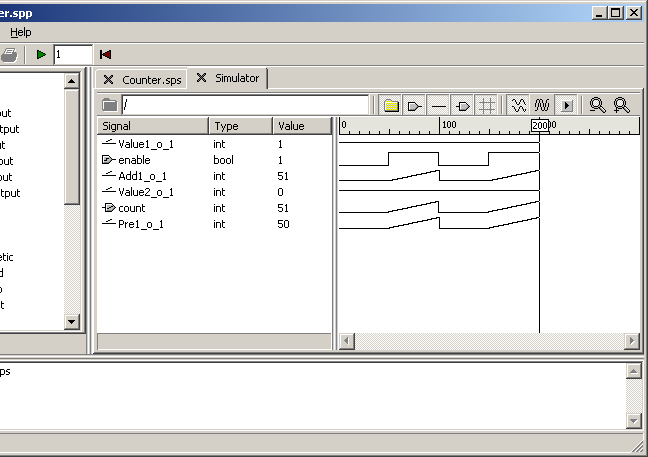
Individual signal values can be forced to any value during the simulation by clicking in the Value or the Force column. For boolean signals, the value will switch between 0 and 1 when clicked, while for other types, a box appears where a new value can be entered. Forcing is removed by right-clicking the value and choosing Unforce in the context menu that appears.
The cursor is a vertical line that is always present in the graph area, by default at the right end of the graphs. However, the cursor can be moved by clicking in the graph area or by pressing Ctrl-Left arrow or Ctrl-Right arrow. The values shown in the signal area always reflect the values at the cursor's position.
Simulated signal values can also be viewed in the schematic right by the corresponding connections. As with the signal area, the schematics reflect the values of the cursor, even if the cursor is not explicitly visible.
A common way to perform simulation is to set up a testbench where input data is fed automatically into the model. In RTflow, this can be done by using the model as a block in another schematic and connecting this block to a signal generator.
The above procedure exemplifies how models can be structured into a hierarchy of schematics. A typical model has a top-level schematic containing the model's inputs and outputs and a number of connected user-defined blocks. These blocks have been defined in schematics that may again contain other user-defined blocks. The definition of a block can be opened by double-clicking it, and one can return to the parent schematic by clicking the Pop Context toolbar button in the schematic editor.
Since the simulator is now set up to simulate the Counter schematic, it is necessary to change this setting to simulate the Testbench schematic and restart the simulator.
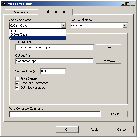
RTflow can generate C, C++, Java and VHDL code from the model, so that it can be implemented in both software and hardware in a real-world application. First of all, you must supply a code generation template in the target language with special keys (e.g. %OUTPUT_UPDATE_EQUATIONS%) indicating where the generated information should be inserted. The code generator reads the template file and makes a copy of it, but where all keys have been replaced with the corresponding information or code. Default template files for all four target languages are supplied with RTflow and can be found under the Templates folder in the application folder.
This tutorial provides a closer look into the simulator by explaining how to use the simulator to tune the parameters of a PID controller. The PID controller and a model of the physical system are already defined in an example project that came with the installation of RTflow, so there is no modeling work involved in this tutorial. Instead, you will iteratively modify the controller parameters and run simulations until a satisfying step response has been achieved. Notice that a basic knowledge of PID controllers is helpful for fully understanding this tutorial.
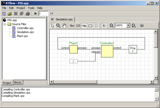
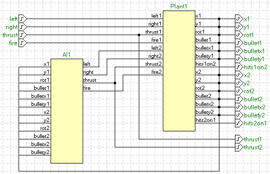
This schematic is the top-level schematic for simulation. It shows clearly how the controller (Controller1) is connected to a model of the physical system (Plant1) in a closed loop. Typically, it is the controller block that is the top-level block for code generation. The physical system model block is only active during simulation, and describes how a real physical system would react to the control value. The physical system model in this example is quite arbitrary (it contains some gain, offset, delay and integration - common elements in a typical system model), and should for the purpose of this tutorial be considered as a black box.
The Pre block between the controller and the plant can be seen as a model of the slight electrical delay of the control signal as it flows from the controller to the physical system. More importantly, however, it prevents the closed loop from becoming a causality loop, that is, a set of blocks that are connected in a loop with no delay. Causality loops are forbidden in RTflow, because it may be difficult or impossible to compile them into executable code. Since the controller contains data paths without delays, and the physical system is a black box that could potentially also contain data paths without delays, a Pre block must be inserted to ensure that there is a delay in the loop.
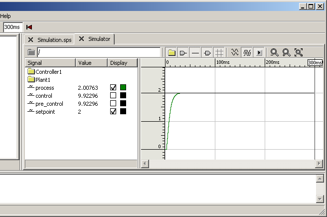
As can be seen, the setpoint to the controller is 2. Therefore, if the controller is tuned properly, we can expect that the process value stabilizes at 2 after some time. The goal of this tutorial is to use the simulator in RTflow to tune the controller further, so that process stabilizes more quickly.
First we will see how the controller performs with the current parameters.
The default display settings of the simulator view are not ideal for studying the simulation output. However, there are a number of possibilities for setting up the display.
RTflow offers two different views for displaying a number of signals: Split view, which shows each graph individually on its own row, and joint view, which shows all signals in one common coordinate system. In split view, the graphs will always be vertically scaled automatically to fit into its narrow row. In joint view, the graphs will be automatically scaled so that all graphs fit into the view. However, in joint view, it is possible to zoom vertically.
By using the checkboxes by the signals' names in the signal area, it is possible to choose the graphs to be displayed in joint view. A maximum of three graphs can be viewed at the same time. For details, see the The Display Column section. When adding or removing a graph, the graph area will be rescaled so that all of the graphs in the new set fit into the view.
Each graph can be given an individual color.
You can freely resize and remove columns in the signal area and resize the graph area to get a better view.
Now that the view is properly set up, we focus our attention on tuning the controller to see if it can perform better. Looking at the results of the simulator, we can see that it takes almost 20 milliseconds to reach a process value over 1.8. This time vill serve as the step response time. Moreover, we can see that after 300 milliseconds, the process value is still not exactly 2, but 2.00763, and very slowly decreasing. Our objective by tuning the controller is to reduce the step response time and to ensure that the process value reaches (and stays at) 2 sooner.
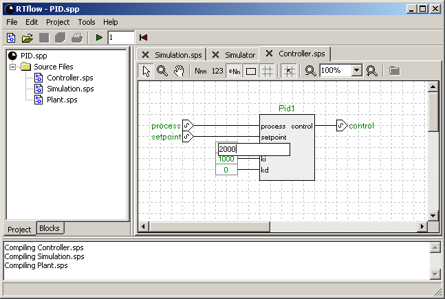
The PID parameters kp, ki and kd can be seen as the inputs to the Pid1 block, and that these values are 1000, 1000 and 0, respectively. To tune the controller, it will suffice to modify these values in this schematic.
If you change the model while the simulation is still running and then invoke the Simulate/Run command (F9), you will be asked if you want to apply the changes and restart the simulation. If you answer Yes, the model will be compiled automatically, and the simulation will restart at time 0. If you answer No, the old simulation will continue without your recent changes. It is not possible to continue the old simulation using the new model.
There are many possibilities for zooming in and out of the graph, so that you can study parts of it at a higher resolution. The Zoom In toolbar button zooms in horizontally around the cursor (the vertical line going through the graph area). The Zoom Out toolbar button zooms out horizontally. By dragging with the mouse inside the graph area, you can create a rectangle into which the graph will zoom when you release the mouse button. Right-clicking in the graph and selecting Zoom Out Vertically in the context menu that appears will zoom out so that the complete vertical extension of all graphs is in view. See the Joint View section for details. Finally, clicking the Restore Zoom toolbar button zooms out both vertically and horizontally so that one pixel corresponds to one cycle.
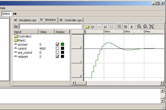
Keep fine-tuning the controller until you are satisfied. You should be able to achieve a step response time at about 7 milliseconds, while the overshoot is no more than 10% (that is, 2.2). As a hint, try applying a small amount of derivative gain using the kd input of the PID block.
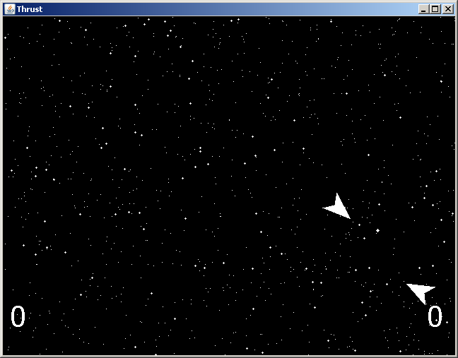
This tutorial shows how RTflow can be used for development of desktop software, in this case a Java game. In this game, you control a spaceship, subject to gravity and physical laws that make it quite challenging to control, and you will try to shoot down an enemy spaceship, controlled by the computer. For the implementation of the game, Java is used for the player interface such as keyboard handling and graphics, while RTflow is used for the physics engine and the artificial intelligence (AI) of the enemy spaceship. The tutorial doesn't present many new features, but it gives you a good and entertaining opportunity to try out some serious development with RTflow.
You don't need a complete Java development environment on your computer to run and develop the game, but you do need the Java development kit (JDK), if you don't already have it. Moreover, it is recommended that you set your PATH user variable to point to the JDK bin folder, so that the java compiler can be called without specifying an absolute path.
A Java (or any kind of) application can be invoked directly from within RTflow using the post-generate command setting in the code generation settings dialog. The post-generate command specifies an executable file, a batch file or a system command to be executed after code generation. For example, the post-generate command can be a batch file that first compiles the generated Java file and then runs the compiled Java application.
javac -sourcepath src -d classes src\rtflow\*.java src\thrust\*.java
java -classpath classes thrust.MainThe AI that controls the enemy ship in this example project is very simple, as can bee seen when trying out the game. In this tutorial, your task is to improve and refine the AI to the level that you think is appropriate. To your help, you have the reference sections in the help system.
A good way to get started would be to create a new AI block by copying the inputs and outputs of the existing AI block:
Your own AI block is now ready to be filled out with logic. At any time, you can press F10 to test the game. Notice, however, that the code generator will fail as long as any of the four output ports of your AI schematic is unconnected. At least you will have to connect them to Value blocks to be able to start the game.
This chapter gives an overview of the main window, followed by a detailed reference of all commands available via the menus, the toolbar buttons, the project tree and the keyboard shortcuts. The sections in this chapter are:
The main window consists of five main parts: The menu bar at the top, the toolbar immediately below, the tree view in the left part of the window, the message view in the bottom, and finally the tab area that occupies the main part of the window. Above the message view, and between the tree view and the tab area, there are separators that can be dragged with the mouse to resize or hide the different parts.
The menu bar allows you to invoke commands. These commands are described in detail in the following sections, sorted under what menu they can be found in. Many commands are also available as toolbar buttons and as keyboard shortcuts, and these are summarized in the Main Window Toolbar Buttons and Main Window Keyboard Shortcuts sections.
It should be noticed that some commands are only available in certain states of the application. For example, Cut is only available if some kind of editor is open and some elements are selected in this editor.
The commands available as toolbar buttons are listed in the Main Window Toolbar Buttons section.
The tree view in the left part of the window can show two different trees depending on what tab has been selected at the bottom of the view. The project tree shows the list of source files in the project, and the commands available on the project tree are listed in the The Project Tree section. The blocks tree is an integral part of the schematic editor and will be described in the The Blocks Tree section.
The message view shows textual messages from various functions in RTflow, including the compiler and the simulator. Compiler error messages commonly includes a link to the failing element, shown in brackets (< and >) and in blue color instead of the ordinary black text. These links can be clicked to open the containing schematic and select the failing element.
The tab area is the main area of the window where source file editors and the simulator view open. Each editor and the simulator is associated to a tab at the top of the area such as when the tab is clicked, the contents are brought into view. Clicking the cross in a tab closes it. Right-clicking a tab brings up a context menu with the Close and Close All commands. Refer to the help sections for these commands for details.
Creates a new schematic. The new schematic is added to the currently open project, and it is opened for editing under a new tab in the tab area. No file is created on disk; the schematic is only opened in memory, and it obtains a temporary filename until you explicitly save it to disk.

Ctrl-N
Always available.
Opens an existing file. A file dialog appears, where you select an existing file. If the selected file is a project file (*.spp), then the currently open project and all open tabs will first be closed as with the Close All command, and then the selected project is opened. If the selected file is a schematic file (*.sps), then the schematic will be opened for editing under a new tab in the tab area.
It should be noticed that when opening a schematic, it is not added to the project. As a consequence, if the schematic was not in the project before, then it is not possible to compile the schematic into a block for use in other schematics. To use a block that a schematic file defines, the file must be added to the project using the Add Files... command.
Also notice that when opening a schematic that itself uses blocks that are not in the project, then these block instances and the connections to them will be removed in the schematic editor. When this happens, warning messaged will be written to the message view. Study the warning messages to find out what blocks are missing and add the missing blocks to the project using the Add Files... command. Then close the failing schematic file without saving the changes and open it again.

Ctrl-O
Always available.
Opens a recently used file without going through a file dialog. Instead, the files to choose between appear in a submenu under the Open Recent item when it is clicked. See Open... for details on the effect of opening a file.
Always available.
Saves the active file. The active file is the file currently in view in the tab area. If the file is new and hasn't been saved to disk before, a file dialog appears, where you choose a folder and enter a name for the file. Notice that if the file is part of a project, then it is recommended to save it in the same folder as, or in a subfolder of, the project file. If not, the project file will contain an absolute path, which makes it difficult to move the project to another location or another computer.

Ctrl-S
Available when an unsaved file is in view in the tab area.
Saves the active file with a new name. The active file is the file currently in view in the tab area. A file dialog appears, where you choose a folder and enter a name for the file. Notice that if the file is part of a project, then it is recommended to save it in the same folder as, or in a subfolder of, the project file. If not, the project file will contain an absolute path, which makes it difficult to move the project to another location or another computer.
Available when a schematic file is in view in the tab area.
Saves the active project with a new name. A file dialog appears, where you choose a folder and enter a name for the project file. It is recommended to save a project file in the same folder as, or in a parent folder of, all the files that it contains. If not, the project file will contain absolute paths, which makes it difficult to move the project to another location or another computer.
Always available.
Saves all modified files. Modified files can be the project file or open source files. For all modified files that are new and haven't been saved before, a file dialog appears, where you choose a folder and enter a name for the file.

Available if the project or any of the open files have been modified.
Closes the active tab. If the tab is a modified source file, you will be asked whether to save the file to disk before closing. In this case, if the you choose Cancel, the file will stay open.
Ctrl-F4
Closes the project and all open tabs. If one or two files are modified, then for each modified file, you will be asked whether to save the file to disk before closing. If three or more files are modified, then the common save dialog appears, where you can choose with a checkbox for each modified file whether to save it or not. The checked files will be saved when you click OK in this dialog. If you click Cancel in this dialog, the files will stay open.
Always available.
Exports data produced by the simulator to a CSV file. The file will contain one column for each signal in the signals view and one row for each cycle that has been simulated so far.
First, a file dialog appears, where you choose a folder and enter a name for the file. Thereafter, the Export CSV Options dialog appears, where you can choose some options for the format of the file. The file will be produced when you click OK in this dialog.
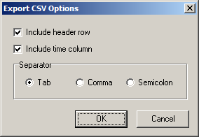
Include header row. When checked, an extra row will be added in the beginning of the file, indicating the names of all signals.
Include time column. When checked, an extra column will be added to the left of the data columns, indicating the cycle number or simulation time in seconds for each row.
Separator. The character to separate the elements with within each row.
Available when the simulator is active in the tab area.
Changes the printer settings. A standard print setup dialog appears, where you can set up printer and page layout settings for source file printing.
Always available.
Prints the schematic if a schematic file is active in the tab area or the graphs if the simulator is active. A standard print dialog appears, where you to set up print parameters. When you click OK, the contents of the active tab is printed.

Ctrl-P
Available when a tab is open in the tab area.
Quits the application. Before the application quits, all files are closed as with the Close All command. If you choose Cancel in any of the save file dialogs that may appear, the exit process aborts and the application will not quit.
Always available.
Reverts the last editing operation. An editing operation is an operation that modifies a source file. Hence, commands like save, compile, and add file can not be undone. Undo never affects the clipboard contents. There is one undo stack for each open source file, so the Undo command will always undo the last action on the currently active file. RTflow supports multi-level undo, which means that a sequence of many editing actions can be undone by using the Undo command repeatedly. The size of the undo stack can be changed with the Options command.
Notice that in the current version of RTflow, undoing a port rename will not properly update other files with references to the port. After undoing a port rename, the schematic should be compiled, and the message view should be inspected for possibly removed connections in other files.
Ctrl-Z
Available if the active tab is a source file and this source file has been modified since it was opened. In addition, the editor must be focused; if it is not, click it to focus it.
Reverts the last undo. Redo never affects the clipboard contents. Since RTflow supports multi-level undo, one can use the Undo and Redo commands to step backwards and forwards in a sequence of many editing operations.
Ctrl-Alt-Z
Available if the active tab is a source file and the Undo command has been used since the last editing operation on the file. In addition, the editor must be focused; if it is not, click it to focus it.
Cuts the selection and puts it on the clipboard.
Ctrl-X
Available if the active tab is a source file and at least one element of the source file is selected. In addition, the editor must be focused; if it is not, click it to focus it.
Copies the selection and puts it on the clipboard.
Ctrl-C
Available if the active tab is a source file and at least one element of the source file is selected. In addition, the editor must be focused; if it is not, click it to focus it.
Inserts clipboard contents. When pasting schematic elements into a schematic, the elements will by default obtain the same position as the original elements. However, pasted elements will always be shifted downwards and to the right so that they don't cover existing copies of the same element. For example, when copying and pasting into the same schematic, the pasted elements will be positioned below and to the right of the original elements. Subsequent pastes will be inserted further down and to the right.
In order to keep the name of every element unique in a schematic, names of copied elements may be augmented with a number.
Ctrl-V
Available if the active tab is a source file and the clipboard contents are compatible with the source file. For schematics, the contents of the clipboard must be schematic elements. In addition, the editor must be focused; if it is not, click it to focus it.
Selects all elements.
Ctrl-A
Available if the active tab is a source file. In addition, the editor must be focused; if it is not, click it to focus it.
Erases the selection. If a block is deleted in a schematic editor, then all connections to and from the block are also deleted.
Del
Available if the active tab is a source file and at least one element of the source file is selected. In addition, the editor must be focused; if it is not, click it to focus it.
Changes properties of the selected element. A window appears, where you can edit properties of the selected element. The window is non-modal, which means that you can still interact with the main window while the Properties window is open. If another element is selected while the Properties window is open, the window will change its contents to show the properties for the new element. If no element is selected, the properties for the entire source file will be shown.
The controls in the Properties window are different depending on what type of element is selected. Descriptions of available properties for schematics and schematic elements are given in the Properties section.
Clicking the OK button applies the chosen property values to the selected element and closes the dialog. Clicking the Apply button applies the chosen property values to the selected element but leaves the dialog open. Finally, clicking the Cancel dialog closes the dialog without applying the values.
Alt-Enter
Available if the active tab is a source file. In addition, the editor must be focused; if it is not, click it to focus it.
Adds files to the project. A source file must be added to the project if the block that it defines is to be used in other schematics. When this command is invoked, a file dialog appears, where you select files to be added. When you click OK in the file dialog, the selected files are added to the project tree, and they are also compiled, so the blocks that they define appear in the blocks tree.
Ctrl-+
Always available.
Removes the active file from the project. Notice that when a file is removed from a project, the block that it defines is also removed. As a consequence, if there are instances of the removed block in another file in the project, then those instances will also be removed, and the project will be invalid. Therefore, it is important to ensure that the block to remove is not used anywhere before proceeding with this command. This can be checked with the Find Usages command.
The file will not be removed from disk, and it will not be closed.
Available if the active tab is a source file in the project.
Compiles the active file. The main reason for using the Compile command is to create or update a block in the blocks tree. There is no reason to use the Compile command for simulation or code generation, since all relevant files will be compiled automatically in those functions.
First, if the file is a schematic file that hasn't been compiled before, then you will be asked for a name for the block that will be created. This name must adhere to the following rules:
Next, the file is checked for syntactic and semantic errors. If errors are found, they will be output to the message view. Some error messages include a link that can be clicked to have the failing element selected in the source file. Refer to the Compiler Errors section for information about error messages.
If no errors are found, a block is created and added to the blocks tree under the User folder. If the file had already been compiled to a block before, then that block is replaced with the new one.
Finally, all open source files are scanned for instances of the block to ensure that they match the new definition. Hence, if the interface of the block was changed (that is, inputs or outputs were added or removed), then all existing instances of the block in open source files will be updated. In addition, connections to removed inputs or outputs will be removed, and for each removed connection, a message will be printed into the message view.
As an example of the above situation, consider two schematics A and B, where the block defined by B is used in A. In A, all the inputs and outputs are connected. Now, if you remove an input port i from the schematic B and then compile B, then the instance of block B in schematic A will be updated accordingly. Hence, the port i will be removed from that instance, and so will the connection to it.
Notice that no files will be changed on disk as a result of the Compile command. If connections are removed from a schematic as in the above example, then those changes take place only in memory. Hence, if you close the modified schematic without saving, then the connections will still be present in the file. Similarly, files that are not open will not be modified. However, as soon as a schematic file is opened, its block instances will be updated to match the current blocks.
F11
Available if the active tab is a source file in the project.
Starts or steps forward the simulator. If the simulation is not already started (that is, the simulator view is not open), then the simulation startup procedure is initiated. The first step in the startup procedure is to check whether the simulation settings have been set. If not, you are prompted to do so, and if you accept, the Project Settings dialog is opened with the Simulation page in front. Refer to the Simulation Settings section for a description of available settings. If you don't accept to set up simulation settings, or if you click Cancel in the Project Settings dialog, simulation is aborted.
Next, all modified source files are compiled as necessary, and then a thorough semantic analysis is performed on the whole model. If errors are found, they will be output to the message view. Some error messages include a link that can be clicked to have the failing element selected in the source file. Refer to the Compiler Errors section for information about error messages.
If no errors are found, simulation is started at cycle 0 and the simulator view is opened. Refer to the The Simulator chapter for information on how to use the simulator view.
If the simulation was already started when the Simulate command is invoked, it is first checked whether any source file or the project settings have been modified since the simulation was started. If so, and you accept to restart the simulation in the dialog that appears, the simulation is reset as described in the Reset Simulator section. Otherwise, the existing simulation is stepped forward with the amount of time specified in the simulation time box in the toolbar. The simulation time box is located to the right of the Simulate toolbar button. Simulation time can be specified as number of cycles or, if appended with the time units "s", "ms" or "us", as real time. For example, entering 10 in the simulation time box will make the simulation step forward by 10 cycles each time the Simulate command is invoked, while entering 10 ms will make it step forward by 10 milliseconds. The real time corresponding to one cycle can be set up in the Simulation Settings.


F9
Available if there is at least one source file in the project.
Resets the simulator. If any source file has been changed since the simulation was started, then the whole model is rebuilt as described in the Simulate section. If no errors are found, all simulated data is erased and simulation is restarted at cycle 0.
If there were forced signals in the simulator before the simulator is reset, then you are asked whether these force settings should be kept. If you reply Yes, these force settings are immediately applied in the new simulation. If you reply No, the force settings are discarded.

Available if the simulator is started.
Generates implementation code. The first step in the code generation procedure is to check whether the code generation settings have been set. If not, you are prompted to do so, and if you accept, the Project Settings dialog is opened with the Code Generation page in front. Refer to the Code Generation Settings section for a description of available settings. If you don't accept to set up code generation settings, or if you click cancel in the Project Settings dialog, code generation is aborted.
Next, all modified source files are compiled as necessary, and then a thorough semantic analysis is performed on the whole model. If errors are found, they will be output to the message view. Some error messages include a link that can be clicked to have the failing element selected in the source file. Refer to the Compiler Errors chapter for information about error messages.
If no errors are found, code generation is performed. Refer to the The Code Generator chapter for information on how the code generator works. Finally, if a post-generate command has been specified in the Project Settings dialog, then this command will be executed.
F10
Available if there is at least one source file in the project.
Finds usages of the block defined by the currently open source file in other source files. The result is output in the message view. First, the number of usages is provided. Then, links to all usages of the block are listed.
Ctrl-U
Available if the active tab is a source file in the project.
Finds blocks in the project that are not used in any source files. Links to all source files that define unused blocks are listed in the message view. Notice that the top-level schematic is considered unused since it, by definition, is not used in any other source, although it may be used for simulation or code generation.
Available if there is at least one source file in the project.
Changes settings for the project. The Project Settings dialog appears, where you can set up settings related to the project. For descriptions of settings under the Simulation tab, refer to the Simulation Settings section. For settings under the Code Generation tab, refer to the Code Generation Settings section.
Clicking the OK button applies the chosen settings to the project and closes the dialog. Clicking the Apply button applies the chosen settings to the project but leaves the dialog open. Finally, clicking the Cancel button closes the dialog without applying the settings.
Notice that project settings are saved with the project file. Hence, if you change a project setting, the project file will be considered modified, and you will be prompted to save the project file if trying to close it without having saved it first.
Always available.
Changes user options for the environment. The Options dialog appears, where you can set up options related to the RTflow application.
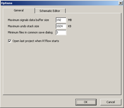
Maximum signals data buffer size. The size in megabytes that the simulator data buffer is allowed to grow to. The simulator will halt when it needs more memory than this to store the simulation result. Increase this value to allow the simulator to run further.
Maximum undo stack size. The size in kilobytes of the editor undo stack. Increase this value to be able to undo more editing operediting operations.
Minimum files in common save dialog. The minimum number of files that must be modified if the common save dialog (described in the Close All section) is to be used, rather than prompting to save each modified individually, when the project is closed. Increase this value to avoid getting the common save dialog when only a few files have been modified.
Open last project when RTflow starts. When checked, RTflow will open the last opened project on startup.
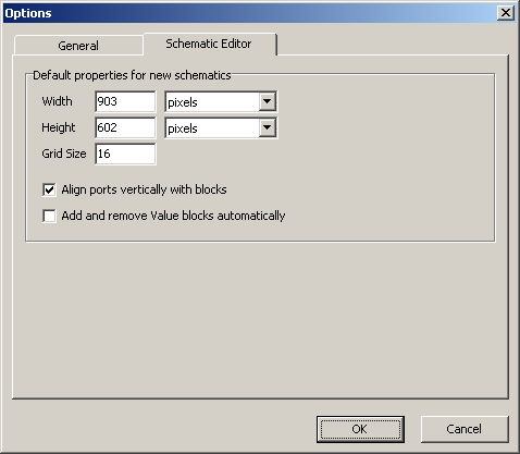
Default properties for new schematics. These options determine the schematic properties for all new schematics that are created with the New Schematic command. Refer to the Schematic Properties section for information about these properties.
Always available.
Opens help.
F1
Always available.
Shows version information.
Always available.
Some commands are available as toolbar buttons in the toolbar immediately under the menu bar. These commands are summarized in the following table.
| Toolbar Button | Command | Description |
|---|---|---|
|
New Schematic | Creates a new schematic. |
|
Open... | Opens an existing file. |
|
Save... | Saves the active file. |
|
Save All | Saves all modified files. |
|
Print... | Prints the active file. |
|
Simulate | Starts or steps forward the simulator. |
|
Simulation Time Box | The number of cycles, or the time, to simulate. |
|
Reset Simulator | Resets the simulator. |
The project tree displays the structure and the members of the project. The top-most node represents the project itself, and therefore it carries the name of the project file. The project node is followed by the Source Files folder that contains one node for each source file in the project. Double-clicking a source file node opens that file for editing. Moreover, right-clicking a node may bring up a context menu with commands that affect the file associated with the node.
Right-clicking the project node brings up a context menu with the following commands:
| Command | Description |
|---|---|
| Add Files... | Adds files to the project. |
| Simulate | Starts or steps forward the simulator. |
| Generate Code | Generates implementation code. |
| Settings... | Changes settings for the project. |
Right-clicking a source file node brings up a context menu with the commands summarized in the following table. Notice that the commands in this menu affect the associated source file, and not the active file, as stated in the detailed reference for the commands. As a consequence, the commands in this menu are always available (that is, never disabled).
| Command | Description |
|---|---|
| Open | Opens the source file. |
| Remove | Removes the source file from the project. |
| Compile | Compiles the source file. |
Some commands are available as keyboard shortcuts. These commands are summarized in the following table.
If the schematic editor is open, additional keyboard shortcuts for editing operations are available. These shortcuts are listed in the Schematic Editor Keyboard Shortcuts section.
| Shortcut | Command | Description |
|---|---|---|
| Ctrl-N | New Schematic | Creates a new schematic. |
| Ctrl-O | Open... | Opens an existing file. |
| Ctrl-S | Save | Saves the active file. |
| Ctrl-F4 | Close | Closes the active tab. |
| Ctrl-P | Print... | Prints the active file. |
| Ctrl-Z | Undo | Reverts the last editing operation. |
| Ctrl-Alt-Z | Redo | Reverts the last undo. |
| Ctrl-X | Cut | Cuts the selection and puts it on the clipboard. |
| Ctrl-C | Copy | Copies the selection and puts it on the clipboard. |
| Ctrl-V | Paste | Inserts clipboard contents. |
| Ctrl-A | Select All | Selects all elements. |
| Alt-Enter | Properties... | Changes properties of the selected element. |
| Ctrl-+ | Add Files... | Adds files to the project. |
| F11 | Compile | Compiles the active file. |
| F9 | Simulate | Starts or steps forward the simulator. |
| F10 | Generate code | Generates implementation code. |
| Ctrl-U | Find Usages | Finds usages of the active file. |
| F1 | Help | Opens help. |
This chapter provides detailed documentation of schematics and the schematics editor. The sections in this chapter are:
A schematic is a sheet containing blocks, connections and other graphical elements that define the behavior of a system model or a sub-component of the system model. In RTflow version 1.1, schematics are the only kind of source files, so the model is always completely defined by a set of schematic files. Schematic files have the extension .sps.
Schematics open in a schematic editor, which appears under a new tab in the tab area. A schematic file can be created or opened for editing in several ways:
This section describes basic editing operations available by clicking and dragging. These operations are:
A block is added to the active schematic by dragging the block from the blocks tree to the schematic with the mouse. The blocks tree is opened by clicking the Blocks tab in the tree view. Read more about the blocks tree in the The Blocks Tree section.
A block can also be added by right-clicking the block in the blocks tree and selecting Add to Schematic in the context menu that appears, or by selecting the block in the blocks tree and pressing the Enter key.
When the new block instance is added, it will be given an instance name that is unique in the schematic. The instance name will be the block name with a number appended on it. For standard and user blocks, the name is displayed with green text above the block instance, and it can be changed as described in the Renaming an Element section.
In RTflow, it is not possible to drag empty blocks from the blocks tree into the schematic, as is possible in some similar software. Instead, create a new schematic, add ports to that schematic and compile it. Then the new block will be available in the blocks tree.
A connection, which is a line connecting two port instances in the schematic, is added by first clicking on the first port instance and then on the second port instance, or by dragging with the mouse from the first to the second port instance.
Since port instances are rather small objects in a schematic at 100% zoom, it may be difficult to find the accurate mouse cursor position where one should click to start the connection. To aid in finding this position, a blue square is shown around the port instance when the mouse cursor is over it, and the name of the port is shown beside it.
After having clicked a port instance, the schematic editor is in connect mode, which means that a line is continuously drawn between the port instance and the mouse cursor, and that if you click another port instance, a connection will be created between the two port instances. If you click somewhere else in the schematic when in connect mode, the connection will be cancelled. It is not possible to create open-ended connections in RTflow.
Connections are only allowed between an output port and an input port, and the two ports must have compatible types. If you try to connect two incompatible port instances, for example two input ports, then an error message will appear in red text by the mouse cursor. To resolve type incompatibility problems, it may be necessary to insert a type conversion block - see the documentation for the Bool, Int and Real blocks.
An output port instance can be attached to many connections. If there are two or more connections emerging from the same output port instance, then there will be one or more points, called connection points, where the paths of two connections split. These points are marked in the schematic with a black dot. The set of connections emerging from the same port may appear as one single connection net, but it is important to remember that these are actually all individual connections. For example, if one of those connections is selected and deleted, the other connections will not be affected.
An input port instance can be attached to only one connection. If a connection is made to an input port instance that is already attached to a connection, then the previous connection will be deleted.
When the new connection is added, it will be given a connection name that is unique in the schematic. By default, the name is hidden, but it can be made visible by clicking the Show Connection Names toolbar button or by pressing N. See the Renaming an Element section for details on how to change the connection name and on the rules governing what names are allowed.
A block is resized by dragging its bottom-right corner with the mouse. The correct mouse cursor position for resizing is indicated by that the cursor is changed from the ordinary arrow to a small double-ended diagonal arrow.
Some blocks, including most primitive blocks, can not be resized.
An interior segment of a connection can be moved by dragging it with the mouse in a direction that is perpendicular to the segment. A segment of a connection is a straight part of a connection and can be either horizontal or vertical. An interior segment is a segment that is not attached to a block instance. Notice that only interior segments can be moved, since segments that are attached to a block have their positions fixed by the positions of the port instances.
When the mouse cursor is over a segment that can be moved, it will change from the ordinary arrow to a small double-ended arrow that is either horizontal (for vertical segments, indicating it can be moved horizontally) or vertical (for horizontal segments, indicating it can be moved vertically).
It is not possible to add or remove segments to the connection. The schematic editor will always minimize the number of segments of a connection, given the positions of its port instances and the directions in which they emerge from the port instances.
There are two different ways to rename an element:
By default, connection names are hidden, but they can be made visible by clicking the Show Connection Names toolbar button or by pressing N. In addition, some block instance names are also hidden, but it can be made visible by selecting the element, opening the Properties dialog and changing the Display settings.
Schematic element names (both block instance and connection names) must adhere to the following rules:
In addition, connection names must adhere to the following rules:
Renaming an input or output port may affect other source files that use the block defined by the edited schematic. In this case, a dialog will appear, listing all affected source files. Clicking OK will perform the name change in the schematic editor and update the references to the port in the listed source files. Open source files will be modified in the editor, while files that are not open will be modified directly on disk. For example, consider two schematics Main.sps and SubFunction.sps, where Main uses SubFunction. If a port name is changed in SubFunction.sps, a dialog will appear, informing that the reference to the port in Main.sps will be modified.
Schematic elements can be selected in several ways:
A block can be moved by dragging it with the mouse. Several blocks can be moved by first selecting them and then dragging one of them with the mouse. Connections attached to the moved blocks will also be moved.
If the Align ports vertically with blocks property is checked in the Schematic Properties, port blocks can not be moved vertically unless the block it is connected to is also moved.
Cutting, copying, pasting and deleting blocks and connections are performed by first selecting the elements and then invoking the command, either from the Edit menu or by using the command's shortcut. For details, refer to the Cut, Copy, Paste and Delete commands.
The schematic editor has a toolbar, situated above the schematic and below the tabs, where you can change functionality and display settings of the schematic editor. The settings apply to all schematic editors and are saved with the user options. The toolbar buttons are summarized in the following table, and the commands that they invoke are described in detail in the subsequent subsections.
| Toolbar Button | Command | Description |
|---|---|---|
 |
Select Tool | Enables the select tool. |
 |
Zoom Tool | Enables the zoom tool. |
 |
Scroll Tool | Enabled the scroll tool. |
 |
Show Connection Names | Shows or hides all connection names. |
 |
Show Values | Shows or hides the simulation values of all signals. |
 |
Show Port Names | Shows or hides port names. |
 |
Show Frame | Shows or hides the frame. |
 |
Show Grid | Shows or hides the grid. |
 |
Snap to Grid | Enables or disables snapping of schematic elements to the grid. |
 |
Zoom Out | Decreases the zoom level. |
 |
Zoom Level | Sets the zoom level. |
 |
Zoom In | Increases the zoom level. |
 |
Pop Context | Opens the source file from which this schematic was opened. |
Enables the select tool. When the select tool is enabled, which it is by default, you can use the mouse to select, add, move and resize elements. The select tool is one of three available tools, of which exactly one is enabled at a time.
S
Always available.
Enables the zoom tool. When the zoom tool is enabled, you can zoom onto a specific point by clicking with the mouse. This is equal to the Zoom In command, but the zoom in point is the point under the cursor, rather than the point in the middle of the view. In the same way, clicking while holding the Ctrl key down zooms out from the point under the cursor. Moreover, you can drag a rectangle over the schematic to zoom such that the area inside the rectangle will cover the view.
Z
Always available.
Enables the scroll tool. When the scroll tool is enabled, you can scroll the schematic by dragging it with the mouse. The scroll tool is one of three available tools, of which exactly one is enabled at a time.
R
Always available.
Shows or hides all connection names. When the button is down, connection names are shown above all connections. When the button is up, connection names are not shown.
N
Always available.
Shows or hides the simulation values of all signals. When the button is down, signal values calculated by the simulator are shown by their corresponding connections. When the button is up, signal values are not shown.
Notice that the simulator must be started for signal values to be sensible. Moreover, you should ensure that the schematic shows the values of the correct instance. This is accomplished by opening the top-level schematic and then double-clicking block instances until the wanted block instance has been reached. The path to the instance will then be shown in the toolbar, to the right of the Pop Context toolbar button, and only then the displayed signal values can be trusted.
V
Always available.
Shows or hides port names. When the button is down, port names are shown by each port instance in the schematic, but only on block instances that are set to display port names. The setting for whether a block instance displays port names can be found in the Block Instance Properties. When the button is up, port names are not shown.
P
Always available.
Shows or hides the frame. When the button is down, the frame of the schematic is shown. When the button is up, the frame is not shown. See the Schematic Properties button for details on frames.
F
Always available.
Shows or hides the grid. When the button is down, a light gray grid is shown on the schematic sheet, so that schematic elements can be aligned more easily. When the button is up, the grid is not shown.
G
Always available.
Enables or disables snapping of schematic elements to the grid. When the button is down, all elements will automatically be snapped to the grid when they are added, moved or resized. Block instances will be moved so that the upper left corner of the block will coincide with a corner of a square in the grid. Connection segments will be moved to the nearest grid line. No elements are moved when this command is invoked; grid snapping only has effect when operating on an element.
T
Always available.
Decreases the zoom level. Zoom level will be set to the preceding zoom factor in the list of predefined zoom factors: 25%, 50%, 75%, 100%, 125%, 150%, 200%, 300% and 400%. For example, if the current zoom level is 180%, pushing the Zoom Out button will set the zoom level to 150%. If possible, the schematic will be scrolled in the view such that the point in the center of the view before zooming out is also in the center of the view afterwards.
F2
Available if the current zoom level is greater than 25%.
Sets the zoom level. A zoom factor can be chosen in the drop-down listbox, or it can be entered by typing in the boxed, followed by an Enter key press. The minimum allowed zoom level is 25% and the maximum allowed zoom level is 400%. If possible, the schematic will be scrolled in the view such that the point in the center of the view before zooming is also in the center of the view afterwards.
Always available.
Increases the zoom level. Zoom level will be set to the succeeding zoom factor in the list of predefined zoom factors: 25%, 50%, 75%, 100%, 125%, 150%, 200%, 300% and 400%. For example, if the current zoom level is 180%, pushing the Zoom In button will set the zoom level to 200%. The schematic will be scrolled in the view such that the point in the center of the view before zooming is also in the center of the view afterwards.
F3
Available if the current zoom level is less than 400%.
Opens the source file from which this schematic was opened. This command is only available if the currently active schematic was opened by double-clicking a block instance in another schematic. In that case, this command opens that other schematic. In effect, if this schematic has been reached by double-clicking block instances several times to walk down in the model hierarchy, this command is used to walk back, upwards in the model hierarchy.
X
Available if this schematic was opened by double-clicking a block instance in another schematic.
All toolbar buttons have associated keyboard shortcuts. These shortcuts are summarized in the following table.
| Shortcut | Command | Description |
|---|---|---|
| S | Select Tool | Enables the select tool. |
| Z | Zoom Tool | Enables the zoom tool. |
| R | Scroll Tool | Enabled the scroll tool. |
| N | Show Connection Names | Shows or hides all connection names. |
| V | Show Values | Shows or hides the simulation values of all signals. |
| P | Show Port Names | Shows or hides port names. |
| F | Show Frame | Shows or hides the frame. |
| G | Show Grid (Schematic Editor) | Shows or hides the grid. |
| T | Snap to Grid | Enables or disables snapping of schematic elements to the grid. |
| F2 | Zoom Out | Decreases the zoom level. |
| F3 | Zoom In | Increases the zoom level. |
| X | Pop Context | Opens the source file from which this schematic was opened. |
Schematics and schematic elements have properties that can be edited in the Properties window. The Properties window opens when the Properties... command is invoked. The contents of the window depends on what element is selected as follows:
In all cases, the name of the schematic or the schematic element is shown in the top of the window. Refer to the Renaming an Element section for details on changing names of schematic elements. Changing the name of the schematic itself will automatically change the name of the block that it defines and may affect other source files that use this block. In this case, a dialog will appear, listing all affected source files. Clicking OK will perform the name change and update the references to the block in the listed source files. Open source files will be modified in the editor, while files that are not open will be modified directly on disk.
Schematic properties apply to the currently active schematic, and will be saved in the schematic file. No other schematic will be affected. To set default properties for new schematics, use the Options dialog.
Width. The width of the schematic, given in the unit specified in the drop-down list immediately to the right of the number.
Height. The height of the schematic, given in the unit specified in the drop-down list immediately to the right of the number.
Grid Size. The length in pixels of the sides of the squares that constitute the grid.
Frame File. The full path to the file containing the frame definition, or No frame if no frame has been added. A new frame can be added to the schematic by clicking the Browse... button and selecting a frame file. A frame is an add-on of graphics to schematics, typically used to enhance the appearance of a printed schematic. However, there is no way to create a frame file in the current version of RTflow, so this should be seen as a future feature.
Align ports vertically with blocks. When checked, all port blocks in the schematic are vertically aligned with the port instance it is connected to. As a result, it is impossible to move a port block vertically by dragging it with the mouse, unless the block instance it is connected to is also moved.
Add and remove Value blocks automatically. When checked, a Value block is always inserted automatically as soon as there is an unconnected input port instance in the schematic, and the new Value block is connected to that port instance. Moreover, unconnected Value blocks are always deleted. As a result, you can not add or remove Value blocks manually as with other blocks - this happens automatically under the mentioned conditions.
Input port order. The order in which the input ports will appear on the left side of the block that this schematic defines. Select a port in the list and press the Up or Down buttons below the list to move the port up and down. After changing the order and clicking OK or Apply, the schematic must also be compiled to apply the changes to the block.
Output port order. The order in which the output ports will appear on the right side of the block that this schematic defines. Select a port in the list and press the Up or Down buttons below the list to move the port up and down. After changing the order and clicking OK or Apply, the schematic must also be compiled to apply the changes to the block.
Block instance properties apply to the selected block instance.
Override block default display properties. When checked, the block instance is displayed using the display properties that are set on this page. When unchecked, the block instance is displayed using the default display properties for the block itself. Default display settings for blocks can not be edited in the current version of RTflow.
Display name. When checked, the instance name is displayed by the block instance. If Above block is selected, the name is displayed above the block instance. If Below block is selected, the name is displayed below the block instance.
Display block name. When checked, the name of the block is displayed by the block instance. If Above block is selected, the name is displayed above the block instance. If Below block is selected, the name is displayed below the block instance.
Display port names. When checked, port names are displayed by each port instance of the block instance, provided that the Show Port Names toolbar button is down. If Inside block is selected, the names are displayed in the interior of the block symbol. If Outside block, the name is displayed outside of the block (immediately above the emerging connection, if any).
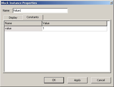
A constant is an input whose value is a constant value specified at design/compile time. For example, the value that you enter in a Value block is a constant for that block. In the current version of RTflow, constants only exist in primitive blocks, and they are all available for editing directly in the schematic by clicking the value inside the symbol. However, to accommodate for future blocks with so many constants that they can't be edited directly in the schematic, constant values for a block instance can also be edited in the Constants page.
There are no properties for connections.
There are no properties for ports.
The blocks tree is the container of all available blocks for use in the schematic editor, available under the Blocks tab in the tree view in the left part of the main window. The blocks are organized in a tree, rather than in a list, in order to facilitate navigation. On the first level of subdivision, all blocks are categorized into one of four different kinds of blocks, as follows:
In the current version of RTflow, there is no way to reorganize the blocks tree. The only modifications that are possible are to add and remove blocks of the User folder. User blocks are added by adding a new schematic to the project and compiling it, and a user block is deleted by removing its source file from the project.
Right-clicking a block in the blocks tree brings up a context menu with the following commands:
| Command | Description |
|---|---|
| Add to Schematic | Adds an instance of the block to the currently active schematic. |
| Edit Source | Opens the source file that defines the block. |
Adds an instance of the block to the currently active schematic. The block instance will be placed in an unoccupied area of the schematic, if possible. For details on adding blocks to schematics, see the Adding a Block section.
Available if the currently active tab in the tab area is a schematic.
Opens the source file that defines the block.
Available if the block is a standard or user block.
This chapter provides detailed documentation of all built-in blocks in RTflow. The sections in this chapter are:
| Name | Symbol | Description |
|---|---|---|
| BoolInput |  | Boolean input port. |
| BoolOutput |  | Boolean output port. |
| IntInput |  | Integer input port. |
| IntOutput |  | Integer output port. |
| RealInput |  | Real input port. |
| RealOutput |  | Real output port. |
Boolean input port. When the schematic is compiled, an input port of type bool will be generated for the block.
Ports\BoolInput
| Name | Type | Description |
|---|---|---|
| o | bool | The incoming signal through this port. |
Boolean output port. When the schematic is compiled, an output port of type bool will be generated for the block.
Ports\BoolOutput
| Name | Type | Description |
|---|---|---|
| i0 | bool | The signal to send out through this port. |
Integer input port. When the schematic is compiled, an input port of type int will be generated for the block. Integers are 32-bit signed integers in the simulator, while it is dependent on the target language in the code generator.
Ports\IntInput
| Name | Type | Description |
|---|---|---|
| o | int | The incoming signal through this port. |
Integer output port. When the schematic is compiled, an output port of type int will be generated for the block.
Ports\IntOutput
| Name | Type | Description |
|---|---|---|
| i0 | int | The signal to send out through this port. |
Real input port. When the schematic is compiled, an input port of type real will be generated for the block. Reals are 32-bit IEEE floating point values in the simulator, while it is dependent on the target language in the code generator.
Ports\RealInput
| Name | Type | Description |
|---|---|---|
| o | real | The incoming signal through this port. |
Real output port. When the schematic is compiled, an output port of type real will be generated for the block.
Ports\RealOutput
| Name | Type | Description |
|---|---|---|
| i0 | real | The signal to send out through this port. |
| Name | Symbol | Description |
|---|---|---|
| Bool |  | Converts a signal of any type to boolean. |
| Int |  | Converts a signal of any type to an integer. |
| Real |  | Converts a signal of any type to a real. |
| If |  | Selects one of two signals depending on a third boolean signal. |
| Not |  | Inverts a boolean signal. |
| And |  | Computes the logical and of two boolean signals. |
| Or |  | Computes the logical or of two boolean signals. |
| Xor |  | Computes the logical xor of two boolean signals. |
| LeftShift |  | Shifts the bits of an integer to the left. |
| RightShift |  | Shifts the bits of an integer to the right. |
| Add |  | Adds two numeric signals. |
| Sub |  | Subtracts two numeric signals. |
| Mult |  | Multiplies two numeric signals. |
| Div |  | Divides two numeric signals. |
| Mod |  | Computes the modulus of two numeric signals. |
| Sqrt |  | Computes the square root of a real-valued signal. |
| Less |  | Determines whether one numeric signal is less than another one. |
| LessEqual |  | Determines whether one numeric signal is less than or equal to another one. |
| Equal |  | Determines whether one signal is equal to another one. |
| NotEqual |  | Determines whether one signal is different from another one. |
| Greater |  | Determines whether one numeric signal is greater than another one. |
| GreaterEqual |  | Determines whether one numeric signal is greater than or equal to another one. |
| Gain |  | Multiplies a real-valued signal by a constant factor. |
| Identity |  | Copies a signal. |
| Value |  | Constant value. |
| Pre |  | Delays a signal one cycle. |
| Dt |  | The real time of one execution cycle in seconds. |
| Sin |  | Computes the sine of a real-valued signal. |
| Cos |  | Computes the cosine of a real-valued signal. |
| Tan |  | Computes the tangent of a real-valued signal. |
| Arctan |  | Computes the arctangent of a real-valued signal. |
| Arctan2 |  | Computes the angle of a two-dimensional vector. |
| Ln |  | Computes the natural logarithm of a real-valued signal. |
| Exp |  | Computes e raised to the power of a real-valued signal. |
| Pow |  | Computes a real-valued signal raised to the power of another real-valued signal. |
Converts a signal of any type to boolean. If i0 is 0, the resulting boolean signal o will be 0. In all other cases, o will be 1.
Primitive\Types\Bool
| Name | Type | Description |
|---|---|---|
| i0 | any | The signal to convert. |
| Name | Type | Description |
|---|---|---|
| o | bool | The resulting boolean signal. |
Converts a signal of any type to an integer. If i0 is boolean, then the resulting signal o will be 0 or 1. If i0 is real, then the fractional part will be truncated. Hence, 2.8 will be converted to 2, while -2.8 will be converted to -2. Integers are 32-bit signed integers in the simulator, while it is dependent on the target language in the code generator.
Primitive\Types\Int
| Name | Type | Description |
|---|---|---|
| i0 | any | The signal to convert. |
| Name | Type | Description |
|---|---|---|
| o | int | The resulting integer signal. |
Converts a signal of any type to a real. The resulting signal o will be the closest possible value to i0. Notice that there are high integer values that can not be represented exactly by the binary representation of real. Reals are 32-bit IEEE floating point values in the simulator, while it is dependent on the target language in the code generator.
Primitive\Types\Real
| Name | Type | Description |
|---|---|---|
| i0 | any | The signal to convert. |
| Name | Type | Description |
|---|---|---|
| o | real | The resulting real signal. |
Selects one of two signals depending on a third boolean signal. If the boolean signal i2 is 0, o will be equal to i0. If i2 is 1, o will be equal to i1.
Primitive\Logic\If
| Name | Type | Description |
|---|---|---|
| i0 | any | The signal to output if i2 is 0. |
| i1 | any | The signal to output if i2 is 1. |
| i2 | bool | The boolean signal that determine whether to output i0 or i1. |
| Name | Type | Description |
|---|---|---|
| o | any | The selected signal. |
Inverts a boolean signal.
Primitive\Logic\Not
| Name | Type | Description |
|---|---|---|
| i0 | bool | The boolean signal to invert. |
| Name | Type | Description |
|---|---|---|
| o | bool | The resulting inverted signal. |
Computes the logical and of two boolean signals. The resulting signal o is 1 if both i0 and i1 are 1, 0 otherwise.
Primitive\Logic\And
| Name | Type | Description |
|---|---|---|
| i0 | bool | Operand. |
| i1 | bool | Operand. |
| Name | Type | Description |
|---|---|---|
| o | bool | Logical and of i0 and i1. |
Computes the logical or of two boolean signals. The resulting signal o is 1 if any of i0 or i1 is 1, 0 otherwise.
Primitive\Logic\Or
| Name | Type | Description |
|---|---|---|
| i0 | bool | Operand. |
| i1 | bool | Operand. |
| Name | Type | Description |
|---|---|---|
| o | bool | Logical or of i0 and i1. |
Computes the logical xor of two boolean signals. The resulting signal o is 1 if exactly one of i0 or i1 is 1, 0 otherwise.
Primitive\Logic\Xor
| Name | Type | Description |
|---|---|---|
| i0 | bool | Operand. |
| i1 | bool | Operand. |
| Name | Type | Description |
|---|---|---|
| o | bool | Logical xor of i0 and i1. |
Shifts the bits of an integer to the left. Zeroes are shifted in to the right side. This is equal to multiplying by 2 to the power of i1.
Primitive\Logic\LeftShift
| Name | Type | Description |
|---|---|---|
| i0 | int | The integer signal to be shifted. |
| i1 | int | The number of bit positions to shift. |
| Name | Type | Description |
|---|---|---|
| o | int | The resulting shifted signal. |
Shifts the bits of an integer to the right. Zeroes are shifted in to the right side. This is equal to dividing by 2 to the power of i1.
Primitive\Logic\RightShift
| Name | Type | Description |
|---|---|---|
| i0 | int | The integer signal to be shifted. |
| i1 | int | The number of bit positions to shift. |
| Name | Type | Description |
|---|---|---|
| o | int | The resulting shifted signal. |
Adds two numeric signals. The two signals must be of the same type.
Primitive\Arithmetic\Add
| Name | Type | Description |
|---|---|---|
| i0 | numeric | Operand. |
| i1 | numeric | Operand. |
| Name | Type | Description |
|---|---|---|
| o | numeric | The sum of i0 and i1. |
Subtracts two numeric signals. The two signals must be of the same type.
Primitive\Arithmetic\Sub
| Name | Type | Description |
|---|---|---|
| i0 | numeric | The first term of the subtraction. |
| i1 | numeric | The term to subtract from i0. |
| Name | Type | Description |
|---|---|---|
| o | numeric | The difference between i0 and i1. |
Multiplies two numeric signals. The two signals must be of the same type.
Primitive\Arithmetic\Mult
| Name | Type | Description |
|---|---|---|
| i0 | numeric | Operand. |
| i1 | numeric | Operand. |
| Name | Type | Description |
|---|---|---|
| o | numeric | The product of i0 and i1. |
Divides two numeric signals. The two signals must be of the same type.
Primitive\Arithmetic\Div
| Name | Type | Description |
|---|---|---|
| i0 | numeric | The numerator. |
| i1 | numeric | The denominator. |
| Name | Type | Description |
|---|---|---|
| o | numeric | The quotient of i0 and i1. |
Computes the modulus of two numeric signals. The two signals must be of the same type. If they are real numbers, o has the same sign as i0, and the absolute value of o is less than the absolute value of i1.
Primitive\Arithmetic\Mod
| Name | Type | Description |
|---|---|---|
| i0 | numeric | The numerator. |
| i1 | numeric | The denominator. |
| Name | Type | Description |
|---|---|---|
| o | numeric | The modulus of i0 and i1. |
Computes the square root of a real-valued signal.
Primitive\Arithmetic\Sqrt
| Name | Type | Description |
|---|---|---|
| i0 | numeric | Operand. |
| Name | Type | Description |
|---|---|---|
| o | numeric | The square root of i0. |
Determines whether one numeric signal is less than another one. The two signals must be of the same type. The resulting signal o is 1 if i0 is less than i1, 0 otherwise.
Primitive\Arithmetic\Less
| Name | Type | Description |
|---|---|---|
| i0 | numeric | Left operand. |
| i1 | numeric | Right operand. |
| Name | Type | Description |
|---|---|---|
| o | bool | 1 if i0 is less than i1, 0 otherwise. |
Determines whether one numeric signal is less than or equal to another one. The two signals must be of the same type. The resulting signal o is 1 if i0 is less than or equal to i1, 0 otherwise.
Primitive\Arithmetic\LessEqual
| Name | Type | Description |
|---|---|---|
| i0 | numeric | Left operand. |
| i1 | numeric | Right operand. |
| Name | Type | Description |
|---|---|---|
| o | bool | 1 if i0 is less than or equal to i1, 0 otherwise. |
Determines whether one signal is equal to another one. The two signals must be of the same type. The resulting signal o is 1 if i0 is equal to i1, 0 otherwise.
Primitive\Arithmetic\Equal
| Name | Type | Description |
|---|---|---|
| i0 | any | Left operand. |
| i1 | any | Right operand. |
| Name | Type | Description |
|---|---|---|
| o | bool | 1 if i0 is equal to i1, 0 otherwise. |
Determines whether one signal is different from another one. The two signals must be of the same type. The resulting signal o is 1 if i0 is different from i1, 0 if i0 is equal to i1.
Primitive\Arithmetic\NotEqual
| Name | Type | Description |
|---|---|---|
| i0 | any | Left operand. |
| i1 | any | Right operand. |
| Name | Type | Description |
|---|---|---|
| o | bool | 1 if i0 is different from i1, 0 if i0 is equal to i1. |
Determines whether one numeric signal is greater than another one. The two signals must be of the same type. The resulting signal o is 1 if i0 is greater than i1, 0 otherwise.
Primitive\Arithmetic\Greater
| Name | Type | Description |
|---|---|---|
| i0 | numeric | Left operand. |
| i1 | numeric | Right operand. |
| Name | Type | Description |
|---|---|---|
| o | bool | 1 if i0 is greater than i1, 0 otherwise. |
Determines whether one numeric signal is greater than or equal to another one. The two signals must be of the same type. The resulting signal o is 1 if i0 is greater than or equal to i1, 0 otherwise.
Primitive\Arithmetic\GreaterEqual
| Name | Type | Description |
|---|---|---|
| i0 | numeric | Left operand. |
| i1 | numeric | Right operand. |
| Name | Type | Description |
|---|---|---|
| o | bool | 1 if i0 is greater than or equal to i1, 0 otherwise. |
Multiplies a real-valued signal by a constant factor.
Primitive\Arithmetic\Gain
| Name | Type | Description |
|---|---|---|
| i0 | real | The signal to apply gain to. |
| Name | Description |
|---|---|
| gain | The constant value to multiply with i0. |
| Name | Type | Description |
|---|---|---|
| o | real | The product of i0 and gain. |
Copies a signal. This block is only useful if the same signal need to appear with two different names in the simulator or in the generated code.
Primitive\Arithmetic\Identity
| Name | Type | Description |
|---|---|---|
| i0 | any | The signal to copy. |
| Name | Type | Description |
|---|---|---|
| o | any | The resulting copy. |
Constant value.
Primitive\Arithmetic\Value
| Name | Description |
|---|---|
| value | The value. |
| Name | Type | Description |
|---|---|---|
| o | any | The value as a signal. |
Delays a signal one cycle. The output signal o is the value that i0 had in the previous execution cycle. If it's the first execution cycle, the output signal o is the value of the constant initial.
Primitive\Dynamic\Pre
| Name | Type | Description |
|---|---|---|
| i0 | any | The signal to delay. |
| Name | Description |
|---|---|
| initial | The value that the output signal o shall have in the first execution cycle. |
| Name | Type | Description |
|---|---|---|
| o | any | The delayed signal, or initial if it's the first execution cycle. |
The real time of one execution cycle in seconds. This value is set in the Project Settings dialog in RTflow for simulation and code generation, respectively.
Primitive\Dynamic\Dt
| Name | Type | Description |
|---|---|---|
| o | real | The real time of one execution cycle in seconds. |
Computes the sine of a real-valued signal.
Primitive\Trigonometric\Sin
| Name | Type | Description |
|---|---|---|
| i0 | real | Operand in radians. |
| Name | Type | Description |
|---|---|---|
| o | real | The sine of i0. |
Computes the cosine of a real-valued signal.
Primitive\Trigonometric\Cos
| Name | Type | Description |
|---|---|---|
| i0 | real | Operand in radians. |
| Name | Type | Description |
|---|---|---|
| o | real | The cosine of i0. |
Computes the tangent of a real-valued signal.
Primitive\Trigonometric\Tan
| Name | Type | Description |
|---|---|---|
| i0 | real | Operand in radians. |
| Name | Type | Description |
|---|---|---|
| o | real | The tangent of i0. |
Computes the arctangent of a real-valued signal. The resulting signal o will be in the interval [-pi/2,+pi/2].
Primitive\Trigonometric\Arctan
| Name | Type | Description |
|---|---|---|
| i0 | real | Operand. |
| Name | Type | Description |
|---|---|---|
| o | real | The arctangent of i0 in radians in the interval [-pi/2,+pi/2]. |
Computes the angle of a two-dimensional vector. i0 is the y-coordinate of the vector and i1 is the x-coordinate of the vector. The resulting signal o will be the angle of the given vector counterclockwise from the x-axis in radians and in the interval [-pi,+pi]. Notice that the length of the vector must be greater than 0, or a math error will occur.
Primitive\Trigonometric\Arctan2
| Name | Type | Description |
|---|---|---|
| i0 | real | Y-coordinate of the vector to calculate the angle of. |
| i1 | real | X-coordinate of the vector to calculate the angle of. |
| Name | Type | Description |
|---|---|---|
| o | real | The angle of the given vector in radians in the interval [-pi,+pi]. |
Computes the natural logarithm of a real-valued signal.
Primitive\Exponential\Ln
| Name | Type | Description |
|---|---|---|
| i0 | real | Operand. |
| Name | Type | Description |
|---|---|---|
| o | real | The natural logarithm of i0. |
Computes e raised to the power of a real-valued signal.
Primitive\Exponential\Exp
| Name | Type | Description |
|---|---|---|
| i0 | real | Operand. |
| Name | Type | Description |
|---|---|---|
| o | real | e raised to the power of i0. |
Computes a real-valued signal raised to the power of another real-valued signal. i0 is the base and i1 is the exponent.
Primitive\Exponential\Pow
| Name | Type | Description |
|---|---|---|
| i0 | real | The base. |
| i1 | real | The exponent. |
| Name | Type | Description |
|---|---|---|
| o | real | i0 raised to the power of i1. |
| Name | Symbol | Description |
|---|---|---|
| Abs |  | Computes the absolute value of a real-valued signal. |
| Distance |  | Computes the distance between two points. |
| Length |  | Computes the length of a vector. |
| Max |  | Selects the greatest value out of two real-valued signals. |
| Min |  | Selected the smallest value out of two real-valued signals. |
| Negation |  | Negates a real-valued signal. |
| SafeArctan2 |  | Computes the angle of a two-dimensional vector and avoids math errors. |
| SafeDiv |  | Divides two real-valued signals and avoids math errors. |
| Saturation |  | Limits a real-valued signal between a lower and an upper bound. |
| Sqr |  | Computes the square of a real-valued signal. |
| Average |  | Computes the average of a real-valued signal over time. |
| Count |  | Counts the number of cycles that a boolean signal has been 1. |
| D |  | Holds the value of a real-valued signal. |
| Derivative |  | Differentiates a real-valued signal. |
| Integral |  | Integrates a real-valued signal. |
| IntegralWithReset |  | Integrates a real-valued signal and allows resetting. |
| Pid |  | Computes a control value given a setpoint signal and process signal using a PID algorithm. |
| PositiveEdge |  | Detects when a boolean signal switches from 0 to 1. |
| SetReset |  | Stores which out of two boolean signals last had a positive edge. |
| T |  | Computes the elapsed real time. |
| Clock |  | Generates a square wave. |
| Ramp |  | Generates a signal that increases or decreases at a fixed rate. |
| Degrees2Radians |  | Converts an angle in degrees to radians. |
| NormalizeAngle |  | Transposes an angle in radians to the interval [-pi,+pi]. |
Computes the absolute value of a real-valued signal.
Standard\Arithmetic\Abs
| Name | Type | Description |
|---|---|---|
| i | real | Operand. |
| Name | Type | Description |
|---|---|---|
| o | real | The absolute value of i. |
Computes the distance between two points. The points are given as two pairs of real cartesian coordinates (x1,y1) and (x2,y2).
Standard\Arithmetic\Distance
| Name | Type | Description |
|---|---|---|
| x1 | real | X coordinate of first point. |
| y1 | real | Y coordinate of first point. |
| x2 | real | X coordinate of second point. |
| y2 | real | Y coordinate of second point. |
| Name | Type | Description |
|---|---|---|
| d | real | The distance between (x1,y1) and (x2,y2). |
Computes the length of a vector. The vector is given as a pair of real cartesian coordinates (dx,dy).
Standard\Arithmetic\Length
| Name | Type | Description |
|---|---|---|
| dx | real | X component of the vector. |
| dy | real | Y component of the vector. |
| Name | Type | Description |
|---|---|---|
| l | real | The length of the vector (dx,dy). |
Selects the greatest value out of two real-valued signals.
Standard\Arithmetic\Max
| Name | Type | Description |
|---|---|---|
| i0 | real | Operand. |
| i1 | real | Operand. |
| Name | Type | Description |
|---|---|---|
| o | real | The greatest value of i0 and i1. |
Selected the smallest value out of two real-valued signals.
Standard\Arithmetic\Min
| Name | Type | Description |
|---|---|---|
| i0 | real | Operand. |
| i1 | real | Operand. |
| Name | Type | Description |
|---|---|---|
| o | real | The greatest value of i0 and i1. |
Negates a real-valued signal.
Standard\Arithmetic\Negation
| Name | Type | Description |
|---|---|---|
| i | real | The signal to negate. |
| Name | Type | Description |
|---|---|---|
| o | real | The negation of i. |
Computes the angle of a two-dimensional vector and avoids math errors. The vector is given as a pair of real cartesian coordinates (x,y). The resulting signal o will be the angle of the given vector counterclockwise from the x-axis in radians and in the interval [-pi,+pi]. If the length of the vector is 0, the resulting signal o will be 0.
Standard\Arithmetic\SafeArctan2
| Name | Type | Description |
|---|---|---|
| y | real | Y-coordinate of the vector to calculate the angle of. |
| x | real | X-coordinate of the vector to calculate the angle of. |
| Name | Type | Description |
|---|---|---|
| rad | real | The angle of the given vector in radians in the interval [-pi,+pi], or 0 if the length of (x,y) is 0. |
Divides two real-valued signals and avoids math errors. If i1, the denominator, is 0, the resulting signal o will be 0.
Standard\Arithmetic\SafeDiv
| Name | Type | Description |
|---|---|---|
| i0 | real | The numerator. |
| i1 | real | The denominator. |
| Name | Type | Description |
|---|---|---|
| o | real | The quotient of i0 and i1, or 0 if i1 is 0. |
Limits a real-valued signal between a lower and an upper bound. The bounds are given as the real-valued signals min and max, where max must be greater than or equal to min. If value is less than min, the resulting signal limited will be min. If value is greater than max, the resulting signal limited will be max. In all other cases, limited will be value.
Standard\Arithmetic\Saturation
| Name | Type | Description |
|---|---|---|
| value | real | The signal to limit. |
| min | real | The lower bound. |
| max | real | The upper bound. |
| Name | Type | Description |
|---|---|---|
| limited | real | The limited signal. |
Computes the square of a real-valued signal.
Standard\Arithmetic\Sqr
| Name | Type | Description |
|---|---|---|
| i | real | Operand. |
| Name | Type | Description |
|---|---|---|
| o | real | The square of i. |
Computes the average of a real-valued signal over time. Values are only accumulated when enable is 1. Before any values have been accumulated, the resulting signal average will be 0. Notice that since the counter of accumulated cycles may be stored in a 32-bit signed integer, the resulting signal may be invalid after 2147483648 accumulated cycles.
Standard\Dynamic\Average
| Name | Type | Description |
|---|---|---|
| i | real | The value to compute the average of. |
| enable | bool | 1 to accumulate i this cycle, 0 to ignore i this cycle. |
| Name | Type | Description |
|---|---|---|
| average | real | The time average of i, or 0 if enable has not yet been 1. |
Counts the number of cycles that a boolean signal has been 1.
Standard\Dynamic\Count
| Name | Type | Description |
|---|---|---|
| enable | bool | 1 to increase the counter this cycle, 0 otherwise. |
| Name | Type | Description |
|---|---|---|
| count | int | The number of cycles that enable has been 1. |
Holds the value of a real-valued signal. When the boolean input signal set is 1, input signal value is copied to the resulting signal o. When set is 0, the resulting signal o holds the same value since set was 1. Before any value has been set, the resulting signal o is 0.
Standard\Dynamic\D
| Name | Type | Description |
|---|---|---|
| value | real | The value to hold. |
| set | bool | 1 to set o to value, 0 to let o keep the old value. |
| Name | Type | Description |
|---|---|---|
| o | real | The value of the signal value when set was last 1, or 0 if set has not yet been 1. |
Differentiates a real-valued signal. The derivative is computed by taking the difference between i0 at this cycle and the previous cycle and dividing it by the sample time.
Standard\Dynamic\Derivative
| Name | Type | Description |
|---|---|---|
| i0 | real | The signal to differentiate. |
| Name | Type | Description |
|---|---|---|
| o | real | The derivative of i0. |
Integrates a real-valued signal. The integral is computed by multiplying i0 by the sample time and accumulating the result. The integral is 0 in the first execution cycle.
Standard\Dynamic\Integral
| Name | Type | Description |
|---|---|---|
| i0 | real | The signal to integrate. |
| Name | Type | Description |
|---|---|---|
| o | real | The integral of i0. |
Integrates a real-valued signal and allows resetting. The integral is computed by multiplying i by the sample time and accumulating the result. If rst is 1, the integration is reset to 0. The integral is 0 in the first execution cycle.
Standard\Dynamic\IntegralWithReset
| Name | Type | Description |
|---|---|---|
| i | real | The signal to integrate. |
| rst | bool | 1 to reset the integration to 0, 0 otherwise. |
| Name | Type | Description |
|---|---|---|
| o | real | The integral of i since rst was 1. |
Computes a control value given a setpoint signal and process signal using a PID algorithm. A PID controller is used to produce a control signal that brings a process signal, typically a sensor signal from a physical system, as close as possible to a given setpoint value. The control signal is connected so that it controls the process (the physical system) that produces the process signal. The parameters kp, ki and kd specify the amount of proportional, integral and derivative gain, respectively, in the resulting control signal. To set these parameters correctly, some knowledge of PID controllers is required. Notice that the PID block reacts instantaneously to changes in the process signal, which means that it is necessary to include a delay (a Pre block) in the model of the process to avoid causality loops when simulating.
Standard\Dynamic\Pid
| Name | Type | Description |
|---|---|---|
| process | real | The process signal that is to be brought closer to setpoint. |
| setpoint | real | The value that the process value should be brought closer to. |
| kp | real | The amount of proportional gain in the PID algorithm. |
| ki | real | The amount of integral gain in the PID algorithm. |
| kd | real | The amount of derivative gain in the PID algorithm. |
| Name | Type | Description |
|---|---|---|
| control | real | The control signal to control the process. |
Detects when a boolean signal switches from 0 to 1.
Standard\Dynamic\PositiveEdge
| Name | Type | Description |
|---|---|---|
| i | bool | The signal whose positive edges to detect. |
| Name | Type | Description |
|---|---|---|
| o | bool | 1 if i is 1 in this cycle and was 0 in the previous cycle, 0 otherwise. |
Stores which out of two boolean signals last had a positive edge. If set was the last signal to have a positive edge, that is switched from 0 to 1, then the resulting signal o is 1. If reset was the last signal to have a positive edge, then the resulting signal o is 0. If both have a positive edge at the same time, reset (0) will have priority. If no signal has yet had a positive edge, the resulting signal is 0.
Standard\Dynamic\SetReset
| Name | Type | Description |
|---|---|---|
| set | bool | The boolean signal whose positive edges sets the resulting signal o to 1. |
| reset | bool | The boolean signal whose positive edges sets the resulting signal o to 0. |
| Name | Type | Description |
|---|---|---|
| o | bool | 1 if set was the last signal to have a positive edge, 0 otherwise. |
Computes the elapsed real time. The time is accumulated in a floating-point signal that will eventually grow so big that further accumulation does not modify it. Hence, the computed time will become invalid. If 32-bit floats with 23 mantissa bits are used, then this happens at latest after 2^23 execution cycles.
Standard\Dynamic\T
| Name | Type | Description |
|---|---|---|
| t | real | The elapsed real time. |
Generates a square wave. A square wave switches regularly between 0 and 1. The input signal t specifies the period time in execution cycles.
Standard\Generators\Clock
| Name | Type | Description |
|---|---|---|
| t | int | The period time in execution cycles. |
| Name | Type | Description |
|---|---|---|
| o | bool | A square wave with period t. |
Generates a signal that increases or decreases at a fixed rate. The start value is given by the input signal start, and the rate is given by the input signal step in change per execution cycle. Both parameters must be fed by constants in order to obtain a fixed change rate.
Standard\Generators\Ramp
| Name | Type | Description |
|---|---|---|
| start | real | The start value, that is, the value that the output signal will have in the first cycle. |
| step | real | The change for each execution cycle. |
| Name | Type | Description |
|---|---|---|
| value | real | The generated signal. |
Converts an angle in degrees to radians.
Standard\Trigonometric\Degrees2Radians
| Name | Type | Description |
|---|---|---|
| deg | real | The angle in degrees to convert. |
| Name | Type | Description |
|---|---|---|
| rad | real | The converted angle in radians. |
Transposes an angle in radians to the interval [-pi,+pi]. The resulting signal o is i + n*2*pi for some integer n such that o is in the interval [-pi,+pi].
Standard\Trigonometric\NormalizeAngle
| Name | Type | Description |
|---|---|---|
| i | real | The angle to transpose in radians. |
| Name | Type | Description |
|---|---|---|
| o | real | The angle in radians in the interval [-pi,+pi]. |
This chapter provides detailed documentation of the simulator and the simulator view. The sections in this chapter are:
The simulator view, which opens under a special tab in the tab area labeled Simulator when simulation is started, consists of three main parts: The signal area in the left half, the graph area in the right half, and the toolbar above the two areas. Between the signal area and the graph area, there is a separator that can be dragged with the mouse to resize or hide the areas.
In this chapter, a different terminology is used for entities that at first may appear as equivalent. However, while the previous chapter dealt with syntactic elements of the schematic language, this chapter deals with their semantic counterparts - mathematical objects involved in the computation and execution of the model, and this distinction calls for a new set of terms. The following table lists the syntactic elements in the previous chapter and the semantic counterparts used in this chapter:
| Syntactic Element | Semantic Counterpart |
|---|---|
| Schematic | Node |
| Non-primitive block instance | Subnode |
| Primitive block instance | Primitive equation |
| Connection | Signal |
This section describes the settings available under the Simulation page in the Project Settings dialog.
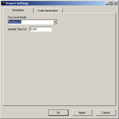
Top-Level Node. The node to be simulated. Naturally, all nodes directly or indirectly used by the top-level node will also be simulated.
Sample Time (s). The real time in seconds corresponding to one execution cycle. This setting specifies the output value of the Dt block, which is used in the definitions of, among others, the Derivative and the Integral blocks. Moreover, it is used to translate real time into execution cycles if you enter a real time value in the simulation time box in the toolbar of the main window. The value must be greater than 0.
The simulator is started and stepped forward by invoking the Simulate command. When the simulator is active, it can be reset by invoking the Reset Simulator command.
The simulator is running as long as the simulator view is open. To stop the simulator, simply close the simulator view.
The signal area shows the state of the simulator as a table. Each row of this table corresponds to one subnode or one signal, and the different columns show different attributes of the signals. When the simulator starts, the signal area shows the subnodes and signals of the top-level node, corresponding to the block instances and connections of the top-level schematic. You can double-click the name of a subnode to enter this node, so that the simulator view shows the subnodes and signals of that node instead. Hence, the signal area works quite similar to the Windows File Explorer, where you double-click a folder to view the contents of it. Therefore, subnodes are symbolized by a folder icon in the signal area.
To optimize the view, you can show or hide individual columns by right-clicking the header row and checking or unchecking the name of the column in the context menu that appears.
The columns of the signal area are:
The Signal column shows the name of the subnode or the signal. To the left of the name, an icon shows the type and kind of the subnode or signal, as follows:
| Icon | Type and kind |
|---|---|
 | Subnode |
 | Boolean input signal |
 | Boolean local signal |
 | Boolean output signal |
 | Integer input signal |
 | Integer local signal |
 | Integer output signal |
 | Real input signal |
 | Real local signal |
 | Real output signal |
Double-clicking a subnode name opens the subnode for viewing in the simulator view.
The Type column shows the type of the signal. Clicking in the Type column has no effect.
The Value column shows the value of the signal at the execution cycle indicated by the cursor. The cursor is the vertical line in the graph area. By default, the cursor is positioned at the end of the simulation data, but it can be moved by clicking in the graph area - see the The Graph Area section for details.
Clicking in the Value column enables forcing of the signal - see the The Force Column section for details on forcing.
The Force column shows whether the signal is currently forced, and to what value. If this column is empty for a signal, then the signal is not being forced, otherwise, it is forced to the shown value.
Forcing means that you override the simulator's computation of a signal and forces it to a specific value. All signals that depend on the forced signal are affected accordingly. It is typically used on input signals in order to see how the model reacts to specific input values, but it is also possible to force local and output signals. Forcing applies immediately to the last cycle of the simulation data and to all cycles being simulated while it is enabled. However, it is not possible to go back and force signals in cycles before the last cycle.
As an example, let's say that you start out by simulating your model for 1000 cycles without any forcing enabled. Hence, the last cycle of the simulation data so far will then be cycle number 1000. Then you force one of the input signals to another value. The value of the input signal itself and all the signals that depend on it will immediately be updated in cycle number 1000, while cycles 0 through 999 will stay unaffected. Finally, you run the simulation for another 1000 cycles, stopping at cycle number 2000. Now all the cycles 1000 through 2000 are affected by the forcing. If you now disable the forcing again, cycle number 2000 will immediately be updated to reflect that no signal is forced, while cycles 1000 through 1999 are still affected by the forcing.
Forcing is enabled by clicking in the Value or the Force column. Depending on the type of the signal, the following happens:
Forcing is disabled by right-clicking the signal and selecting Unforce in the context menu that appears.
The Display column shows the graph display settings for the signal. The column contains two boxes; the visible box and the color box.
The visible box is a check box such that when checked, the signal's graph is visible in the graph area, otherwise it is invisible. It has effect only in joint view. Clicking the check box switches between checked (visible) and unchecked (invisible). At most three graphs can be visible at a time. If you check the visible box of a fourth signal, another signal's visible box will be unchecked, and its graph will accordingly disappear.
The color box shows the color of the graph of the signal. Clicking the color box opens a color picker dialog, where you can choose another color for the graph. Clicking OK in the color picker dialog applies the new color to the graph.
The graph area shows the simulated data as graphs of signal values over time. It can operate in two different modes:
You can switch between split view and joint view using the Split View and Joint View toolbar buttons.
For both views, the horizontal axis is (simulated) time, and the scale is shown in the top of the view. Depending on whether you have specified simulation time as a number of cycles or as real time in the simulation time box in the toolbar of the main window, the scale shows the time either as the number of cycles elapsed or as the real time elapsed accordingly. In the latter case, a time unit is shown in the scale, or, if more than one minute has elapsed, the time is shown as hours, minutes and seconds, separated by colons.
The cursor is a vertical line through the whole graph area. Its exact position is shown in a box in the scale, in the top of the area. By default, the cursor is positioned at the last cycle of the simulated data, but you can move it by clicking in the graph or the scale at the time to which the cursor should be moved. The position of the cursor decides what cycle the values in the Value column are shown for.
In split view, the graph area shows each graph in its own row, which is the extension of the signal's row in the signals view. The vertical scales of the individual graphs adjust automatically, so that the entire graph computed so far fits in the row. Split view is typically used when you want to have an overview of the trends of all signals in view.
If you drag with the mouse horizontally over the graph area, the graphs will zoom in horizontally such that the area covered by the mouse will fill the whole graph area. There is no way to zoom in vertically or increase the height of the rows in split view in the current version of RTflow. To zoom out again, right-click in the graph area and select one of the following:
In joint view, the graph area shows all graphs in the same coordinate system. At most three graphs can be displayed, and these are selected by clicking the visible box in the Display column of the signal in the signal area. By default, the vertical scale adjusts automatically, so that all of the graphs computed so far fit in the area. Joint view is typically used when you want to study the details of a few specific signals.
If you drag with the mouse over the graph area, the graphs will zoom in such that the area covered by the mouse will fill the whole graph area. As a consequence, the automatic vertical scaling is disabled, and further simulation will not rescale the graphs. To zoom out and/or reenable automatic vertical scaling, right-click the graph area and select one of the following:
The simulator view has a toolbar, situated above the signal and graph areas and below the tabs, where you can change functionality and display settings of the simulator view. The toolbar buttons are summarized in the following table, and the commands that they invoke are described in detail in the subsequent subsections.
| Toolbar Button | Command | Description |
|---|---|---|
|
Pop Context | Shows the signals of the supernode of the current instance. |
 |
Current Instance | Shows the path from the top-level node to the current instance. |
 |
Show Subnodes | Shows or hides rows with subnodes in the signal area. |
 |
Show Inputs | Shows or hides rows with input signals in the signal area. |
 |
Show Locals | Shows or hides rows with local signals in the signal area. |
 |
Show Outputs | Shows or hides rows with output signals in the signal area. |
|
Show Grid | Shows or hides the grid in the graph area. |
 |
Split View | Switches the graph area to split view. |
 |
Joint View | Switches the graph area to joint view. |
 |
Auto Scroll | Enables or disables automatic horizontal scrolling of the graph area. |
|
Zoom Out | Decreases the horizontal zoom level of the graph area. |
|
Zoom In | Increases the horizontal zoom level of the graph area. |
 |
Restore Zoom | Restores vertical and horizontal zoom of the graph area to the default setting. |
Shows the signals of the supernode of the current instance. This command is only available if you have double-clicked a subnode in the signal area, so that the signals of a subnode are currently being shown. In that case, this command returns to the parent node. In effect, if the current instance has been reached by double-clicking subnodes several times to walk down in the model hierarchy, this command is used to walk back, upwards in the model hierarchy.
Available when the signal area is showing the signals of another node than the top-level node.
Shows the path from the top-level node to the current instance. The current instance is the node instance (the top-level node or any subnode) whose signals are currently being shown in the simulator view. The path is a sequence of subnode names, separated by slashes, such that one can start from the top-level node and double-click the subnodes specified in the sequence in order to reach the current instance. You can also manually enter a path in the field, but if the entered path is invalid, no signals will be shown.
Always available.
Shows or hides rows with subnodes in the signal area. When the button is down, subnodes of the current instance are shown in the signal area. When the button is up, the subnodes are hidden.
Always available.
Shows or hides rows with input signals in the signal area. When the button is down, input signals of the current instance are shown in the signal area. When the button is up, the input signals are hidden.
Always available.
Shows or hides rows with local signals in the signal area. When the button is down, local signals of the current instance are shown in the signal area. When the button is up, the local signals are hidden. Local signals correspond to connections that are internal in the schematics, that is, not attached to a port block.
Always available.
Shows or hides rows with output signals in the signal area. When the button is down, output signals of the current instance are shown in the signal area. When the button is up, the output signals are hidden.
Always available.
Shows or hides the grid in the graph area. When the button is down, a light gray grid is shown in the graph area, indicating major time units by vertical lines and, if the graph area is in joint view, major value units by horizontal lines. When the button is up, the grid is not shown.
Always available.
Switches the graph area to split view. See the Split View section for a description of the split view.
Available when the graph area is in joint view.
Switches the graph area to joint view. See the Joint View section for a description of the joint view.
Available when the graph area is in split view.
Enables or disables automatic horizontal scrolling of the graph area. When the button is down, invoking the Simulate command for stepping forward the simulator will automatically cause the graph area to scroll horizontally to the end of the simulated data. When the button is up, the graph area will not scroll automatically.
Always available.
Decreases the horizontal zoom level of the graph area. The zoom level is decreased by half, such that the same time interval covers half the horizontal extension after zooming out. If possible, the graph area will also scroll such that the cursor stays at the same screen position.
All elements of the graphs are shown, also in zoom levels of less than one pixel per cycle. For instance, consider a graph of a signal that is 0 for all cycles 0 through 1,000,000, except for one single cycle in the middle, where it is 1. This spike will be seen in the graph, regardless of how far out you zoom. However, a consequence of this feature is that drawing can become slow at very low zoom levels.
Available when the current zoom level is greater than 1/1,000,000 pixels per cycle.
Increases the horizontal zoom level of the graph area. The zoom level is doubled, such that the same time interval covers double the horizontal extension after zooming in. If possible, the graph area will also scroll such that the cursor stays at the same screen position.
Available when the current zoom level is less than 16 pixels per cycle.
Restores vertical and horizontal zoom of the graph area to the default setting. Horizontal zoom is restored to one pixel per cycle. Moreover, if the graph area is in joint view, automatic vertical scaling is reenabled so that all of the graphs computed so far fit in the area.
Always available.
The following table summarizes the keyboard shortcuts available in the simulator.
| Shortcut | Command | Description |
|---|---|---|
| Ctrl-Left arrow | Cursor Back | Moves the cursor one cycle back in the simulation data. |
| Ctrl-Right arrow | Cursor Forward | Moves the cursor one cycle forward in the simulation data. |
Moves the cursor one cycle back in the simulation data. As a consequence, the signal area shows the signal values for the previous cycle. This command can also be used when studying signal values in a schematic editor.
Ctrl-Left arrow
Available when the cursor is not at the first cycle.
Moves the cursor one cycle forward in the simulation data. As a consequence, the signal area shows the signal values for the next cycle. This command can also be used when studying signal values in a schematic editor.
Ctrl-Right arrow
Available when the cursor is not at the last cycle of the simulated data.
This chapter provides detailed documentation of the code generator. The sections in this chapter are:
RTflow can generate implementation code from the model, so that it can be implemented in a real-world application. To be more precise, RTflow can generate C, C++ and Java for software implementations and synthesizable VHDL for FPGA/ASIC implementations. Code generation is performed by invoking the Generate Code command. The first time, you will be asked to set up some code generation settings in the project settings dialog. Subsequent invocations require no further user interaction.
Among a few other settings for code generation, you have to specify a template file. The template file defines the interface of the generated file by means of skeleton functions that contain code generation keys. The code generator reads the template file and outputs a copy of it, but with the keys replaced by actual generated code. Most users don't need to write their own template file, but can use the ones supplied with RTflow - see the table below. However, advanced users may prefer to write their own template file. The Key Reference provides the primary documentation for those users.
The template files supplied with RTflow are (paths are relative to the application folder):
| Target Language | Path |
|---|---|
| C | Templates/Template.c |
| C++ | Templates/Template.cpp |
| Java | Templates/Template.java |
| VHDL | Templates/Template.vhd |
It is recommended to copy the template file to the project folder, to ensure that the project can be moved to other computers.
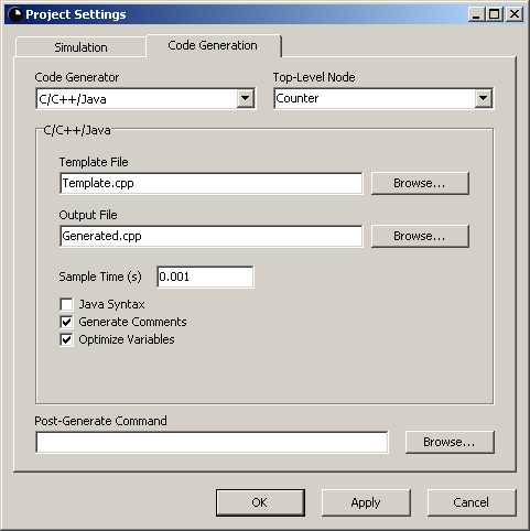
Code Generator. The code generator module to use, and hence, what target language to generate.
Top-Level Node. The node to generate code for. Naturally, code will also be generated for all nodes directly or indirectly used by the top-level node.
Post-Generate Command. A system command, an executable file or a batch file that will be executed after each code generation. In the case of an executable file or a batch file, the path can be both absolute or relative to the project folder, that is, the folder containing the project file. Click the Browse... button to the right of the field to select the executable or batch file using a file dialog.
The remaining settings are dependent on what code generator was chosen in the Code Generator drop-down box. For C/C++/Java, see the C/C++/Java Generator Settings section. For VHDL, see the VHDL Generator Settings section.
Template File. The template file for code generation. See the Code Generator - General section for an explanation of the template file. The path can be both absolute or relative to the project folder, that is, the folder containing the project file. Click the Browse... button to the right of the field to select the template file using a file dialog.
Output File. The location and name of the file to generate. The path can be both absolute or relative to the project folder, that is, the folder containing the project file. Click the Browse... button to the right of the field to select the location and name using a file dialog.
Sample Time (s). The real time in seconds corresponding to one execution cycle. This setting specifies what the %SAMPLE_TIME% key in the template file will be translated to in the code generation. It also specifies the output value of the Dt block, which is used in the definitions of, among others, the Derivative and the Integral blocks. The value must be greater than 0.
Java Syntax. When checked, Java code will be generated instead of C/C++ code. For example, the call to a sine function will be Math.sin(x) instead of just sin(x).
Generate Comments. When checked, each generated assignment will be followed by a comment that indicates what signals are involved in the operation. As an example, i[1] = i[2] + i[3]; could be followed by /* sum = pre_count + v1; */. While this option makes the generated file bigger, it also makes it a little more human-readable.
Optimize Variables. When checked, the generated code will be optimized. As a consequence, some internal signals may be removed. This means that the caller of the generated code can not assume that all signals in the source files will also exist in the code. However, the input and output signals of the top-level node will always be available.
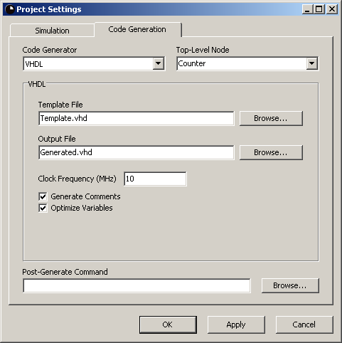
Template File. The template file for code generation. See the Code Generator - General section for an explanation of the template file. The path can be both absolute or relative to the project folder, that is, the folder containing the project file. Click the Browse... button to the right of the field to select the template file using a file dialog.
Output File. The location and name of the file to generate. The path can be both absolute or relative to the project folder, that is, the folder containing the project file. Click the Browse... button to the right of the field to select the location and name using a file dialog.
Clock Frequency (MHz). The frequency in MHz of the clock that will drive the implementation. This setting specifies what the %FREQUENCY_MHZ% key in the template file will be translated to in the code generation. It also determines the output value of the Dt block, which is used in the definitions of, among others, the Derivative and the Integral blocks. The value of Dt will be 1 / (clock frequency * 1,000,000). The clock frequency must be greater than 0.
Generate Comments. When checked, each generated assignment will be followed by a comment that indicates what signals are involved in the operation. As an example, i(1) <= i(2) + i(3); could be followed by -- sum <= pre_count + v1;. While this option makes the generated file bigger, it also makes it a little more human-readable.
Optimize Variables. When checked, the generated code will be optimized. As a consequence, some internal signals may be removed. This means that the caller of the generated code can not assume that all signals in the source files will also exist in the code. However, the input and output signals of the top-level node will always be available.
The following table summarizes the code generation keys that will be recognized in the template file. type can be any of BOOL, INT and REAL. Keys are case sensitive and are always in capital letters. Most of the keys can be used with both the C/C++/Java generator and the VHDL, while a few keys are unique for one of the generators. The table specifies with an X for which code generators the key can be used.
| Key | Description | C/C++/Java | VHDL |
|---|---|---|---|
| %type_VECTOR% | The name of the type array. | X | X |
| %IF_HAS_type% | Includes the line if and only if there are type signals. | X | X |
| %type_NAMES% | The names of the signals and states in the type array. | X | |
| %type_INPUT_NAMES% | The names of the input signals of type type. | X | |
| %type_OUTPUT_NAMES% | The names of the output signals of type type. | X | |
| %NUMBER_type% | The total number of type signals. | X | X |
| %NUMBER_type_INPUT% | The number of type input signals. | X | X |
| %NUMBER_type_OUTPUT% | The number of type output signals. | X | X |
| %NUMBER_type_LOCAL% | The number of type local signals. | X | X |
| %NUMBER_type_STATE% | The number of type state variables. | X | X |
| %OFFSET_type_INPUT% | The index of the first input signal in the type array. | X | X |
| %OFFSET_type_OUTPUT% | The index of the first output signal in the type array. | X | X |
| %OFFSET_type_LOCAL% | The index of the first local signal in the type array. | X | X |
| %OFFSET_type_STATE% | The index of the first state variable in the type array. | X | X |
| %INITIAL_EQUATIONS% | Code that resets all state variables to the initial state. | X | X |
| %OUTPUT_UPDATE_EQUATIONS% | Code that computes all local and output signals from the current inputs and states. | X | X |
| %STATE_UPDATE_EQUATIONS% | Code that transitions the state variables to the next cycle. | X | X |
| %SAMPLE_TIME% | The real time in seconds corresponding to one execution cycle. | X | |
| %FREQUENCY_MHZ% | The frequency in MHz of the clock that will drive the implementation. | X | |
| %INPUT_MAP% | Code that copies input signals from the entity's interface to the arrays. | X | |
| %OUTPUT_MAP% | Code that copies output signals from the arrays to the entity's interface. | X |
The name of the type array. type can be any of BOOL, INT and REAL, such that the actual keys are %BOOL_VECTOR%, %INT_VECTOR% and %REAL_VECTOR%.
Rather than declaring one single variable (in VHDL: signal) for each signal of the RTflow model, the code generator expects the existence of arrays (in VHDL: vectors), in which all signals reside. Hence, the generated code is merely a sequence of computations on elements of these arrays. There must be one array for each of the basic types boolean, integer and real, and it is the template author's responsibility to declare these appropriately. To do this, the array names that are used in the generated code must be known, and these are given by the %type_VECTOR% key.
C/C++/Java, VHDL
%IF_HAS_REAL% public float[] %REAL_VECTOR% = new float[%NUMBER_REAL%];
%IF_HAS_BOOL% signal %BOOL_VECTOR% : std_logic_vector(%NUMBER_BOOL%-1 downto 0);
Includes the line if and only if there are type signals. type can be any of BOOL, INT and REAL.
If this key is found in a line of the template file during code generation, then that whole line will only be processed if the number of variables of type type is greater than 0. This is useful for avoiding declarations of arrays with zero elements, which is forbidden in some target languages.
C/C++/Java, VHDL
%IF_HAS_REAL% public float[] %REAL_VECTOR% = new float[%NUMBER_REAL%];
The names of the signals and states in the type array. type can be any of BOOL, INT and REAL.
If this key is found in a line of the template file during code generation, then that whole line will be copied the same number of times as there are signals of type type, and in each copy, the %type_NAMES% key is replaced by the name of the signal residing in the corresponding cell of the array. As a result, this key generates the complete list of the names of all signals in the type array. This information is used to associate an array index with an actual signal in the RTflow model.
The names of signals in the top-level node are provided without modifications. However, for signals in subnodes, the names are prepended with the instance path to the subnode containing the signal. Hence, if the subnode A is a subnode of the top-level node, and subnode A has a signal i, then that signal will be given the name "A/i" in the generated name list.
C/C++/Java
public String[] boolNames = new String[]
{
   "%BOOL_NAMES%",
   ""
};
The names of the input signals of type type. type can be any of BOOL, INT and REAL.
If this key is found in a line of the template file during code generation, then that whole line will be copied the same number of times as there are input signals of type type, and in each copy, the %type_INPUT_NAMES% key is replaced by the name of an input signal.
An input signal in the code generation context is an input signal of the top-level node. Inputs of subnodes count as local signals.
VHDL
entity RTflowCode is
   port(
      %BOOL_INPUT_NAMES% : in std_logic;
      %INT_INPUT_NAMES% : in integer;
      %REAL_INPUT_NAMES% : in float32;
      %BOOL_OUTPUT_NAMES% : out std_logic;
      %INT_OUTPUT_NAMES% : out integer;
      %REAL_OUTPUT_NAMES% : out float32;
      clk : in std_logic
   );
end RTflowCode;
The names of the output signals of type type. type can be any of BOOL, INT and REAL.
If this key is found in a line of the template file during code generation, then that whole line will be copied the same number of times as there are output signals of type type, and in each copy, the %type_OUTPUT_NAMES% key is replaced by the name of an output signal.
An output signal in the code generation context is an output signal of the top-level node. Outputs of subnodes count as local signals.
VHDL
See %type_INPUT_NAMES%.
The total number of type signals. type can be any of BOOL, INT and REAL.
This key provides the size of the array for each basic type. See %type_VECTOR% for details about the arrays in code generation.
C/C++/Java, VHDL
%IF_HAS_REAL% public float[] %REAL_VECTOR% = new float[%NUMBER_REAL%];
%IF_HAS_BOOL% signal %BOOL_VECTOR% : std_logic_vector(%NUMBER_BOOL%-1 downto 0);
The number of type input signals. type can be any of BOOL, INT and REAL.
An input signal in the code generation context is an input signal of the top-level node. Inputs of subnodes count as local signals.
C/C++/Java, VHDL
The number of type output signals. type can be any of BOOL, INT and REAL.
An output signal in the code generation context is an output signal of the top-level node. Outputs of subnodes count as local signals.
C/C++/Java, VHDL
The number of type local signals. type can be any of BOOL, INT and REAL.
An local signal in the code generation context is any signal that is not an input or an output of the top-level node. Hence, all signals of the subnodes count as local signals in this context.
C/C++/Java, VHDL
The number of type state variables. type can be any of BOOL, INT and REAL.
A state variable is the holder of a value from the previous cycle, corresponding to a Pre block. State variables don't exist explicitly in the abstract RTflow model, but are necessary in the generated implementation code. See %STATE_UPDATE_EQUATIONS% for details about how state variables are used.
C/C++/Java, VHDL
The index of the first input signal in the type array. type can be any of BOOL, INT and REAL.
Each of the arrays (one for each of the basic types boolean, integer and real) is partitioned into input signals, output signals, local signals and state variables. This key provides the index of the first input signal in the array. Hence, the index of the n:th boolean input signal in the boolean array is %OFFSET_BOOLEAN_INPUT% + n.
An input signal in the code generation context is an input signal of the top-level node. Inputs of subnodes count as local signals.
C/C++/Java, VHDL
The index of the first output signal in the type array. type can be any of BOOL, INT and REAL.
Each of the arrays (one for each of the basic types boolean, integer and real) is partitioned into input signals, output signals, local signals and state variables. This key provides the index of the first output signal in the array. Hence, the index of the n:th boolean output signal in the boolean array is %OFFSET_BOOLEAN_OUTPUT% + n.
An output signal in the code generation context is an output signal of the top-level node. Outputs of subnodes count as local signals.
C/C++/Java, VHDL
The index of the first local signal in the type array. type can be any of BOOL, INT and REAL.
Each of the arrays (one for each of the basic types boolean, integer and real) is partitioned into input signals, output signals, local signals and state variables. This key provides the index of the first local signal in the array. Hence, the index of the n:th boolean local signal in the boolean array is %OFFSET_BOOLEAN_LOCAL% + n.
An local signal in the code generation context is any signal that is not an input or an output of the top-level node. Hence, all signals of the subnodes count as local signals in this context.
C/C++/Java, VHDL
The index of the first state variable in the type array. type can be any of BOOL, INT and REAL.
Each of the arrays (one for each of the basic types boolean, integer and real) is partitioned into input signals, output signals, local signals and state variables. This key provides the index of the first state variable in the array. Hence, the index of the n:th boolean state variable in the boolean array is %OFFSET_BOOLEAN_LOCAL% + n.
A state variable is the holder of a value from the previous cycle, corresponding to a Pre block. State variables don't exist explicitly in the abstract RTflow model, but are necessary in the generated implementation code. See %STATE_UPDATE_EQUATIONS% for details about how state variables are used.
C/C++/Java, VHDL
Code that resets all state variables to the initial state.
If this key is found in a line of the template file during code generation, then that whole line will be copied the same number of times as there are state variables of all types, and in each copy, the %INITIAL_EQUATIONS% key is replaced by an assignment statement of a state variable to its initial value. As a result, this key generates the code that should be executed once in the initialization of the process. None of the input, output or local signals are assigned or referred in this code.
C/C++/Java, VHDL
void initialize()
{
   %INITIAL_EQUATIONS%
}
Code that computes all local and output signals from the current inputs and states.
If this key is found in a line of the template file during code generation, then that whole line will be copied the same number of times as there are output and local signals of all types, and in each copy, the %OUTPUT_UPDATE_EQUATIONS% key is replaced by a statement where a local or output signal is computed and assigned. As a result, this key generates the code that, together with %STATE_UPDATE_EQUATIONS%, should be executed for each cycle.
C/C++/Java, VHDL
void run()
{
   %OUTPUT_UPDATE_EQUATIONS%
   %STATE_UPDATE_EQUATIONS%
}
process (clk)
begin
   if reset = '1' then
      %INITIAL_EQUATIONS%
   elsif clk'event and clk = '1' then
      %STATE_UPDATE_EQUATIONS%
   endif;
end process;
%OUTPUT_UPDATE_EQUATIONS%
Code that transitions the state variables to the next cycle.
If this key is found in a line of the template file during code generation, then that whole line will be copied the same number of times as there are state variables of all types, and in each copy, the %STATE_UPDATE_EQUATIONS% key is replaced by an assignment statement of a state variable to a value computed by the last %OUTPUT_UPDATE_EQUATIONS% execution. In schematic terms, this corresponds to that the values of signals connected to the input of Pre blocks are transferred into the memory registers (state variable) that the Pre blocks constitute. As a result, this key generates the code that, together with %OUTPUT_UPDATE_EQUATIONS%, should be executed for each cycle.
C/C++/Java, VHDL
See %OUTPUT_UPDATE_EQUATIONS%.
The real time in seconds corresponding to one execution cycle.
C/C++/Java
public float getSampleTime()
{
   return %SAMPLE_TIME%;
}
The frequency in MHz of the clock that will drive the implementation.
VHDL
Code that copies input signals from the entity's interface to the arrays.
If this key is found in a line of the template file during code generation, then that whole line will be copied the same number of times as there are input signals of all types, and in each copy, the %INPUT_MAP% key is replaced by an assignment statement that copies a VHDL entity input signal to an input signal in the array. The entity input signal has the same name as the corresponding input of the top-level node. Hence, the entity should be declared as in the example for %type_INPUT_NAMES%.
VHDL
process (clk)
begin
   if clk'event and clk = '1' then
      %INPUT_MAP%
   end if;
end process;
Code that copies output signals from the arrays to the entity's interface.
If this key is found in a line of the template file during code generation, then that whole line will be copied the same number of times as there are output signals of all types, and in each copy, the %OUTPUT_MAP% key is replaced by an assignment statement that copies an output signal in the array to a VHDL entity output signal. The entity output signal has the same name as the corresponding output of the top-level node. Hence, the entity should be declared as in the example for %type_INPUT_NAMES%.
VHDL
The following table summarizes error messages that may be output to the message view as a result of a Compile, Simulate or Generate Code command. Detailed descriptions of the cause of these errors and suggestions for how to resolve them are given in the subsequent subsections.
Notice. The compiler may output error messages that are not listed here. There may be two different reasons for this:
There is a causality loop in the model, which means that a set of blocks that are connected in a loop without any delay (Pre) block. Causality loops are forbidden in RTflow, because it may be difficult or impossible to compile them into executable code. The sequence of signals that constitute the loop are given in the error message.
Insert a Pre block anywhere in the loop.
An output port block is not connected to any source, which would leave the output value undefined.
Connect the block to any output port instance, or create a new Value block instance in the schematic and connect it to the output port block.
A schematic contains a block instance of the block that it defines, possibly through other blocks, which causes an infinite recursion. For example, if schematic A contains an instance of block B, and schematic B contains and instance of block A, then the schematics A and B constitute a recursion.
Remove the block instance involved in the recursion from any of the involved schematics.
A schematic file contains an instance of a block that doesn't exist. This can happen if a schematic file has been removed from the project without properly updating other schematics that use the removed block.
Either add the missing schematic file to the project, or open the failing file, in which case the failing block instances will be removed automatically.
An input port instance is not connected to any source, which would leave the input value undefined.
Connect the input port instance to any output port instance, or create a new Value block instance in the schematic and connect it to the input port instance.
A block has been connected to signals of different types, violating a requirement that all connected signals must have the same types. For example, if an Add block is connected to two integer input port blocks and to a real output port block, then a type mismatch occurs, since all ports of the Add block must be connected to signals of the same type.
Insert a type conversion block (Bool, Int or Real) in the failing connection.
The template file given in the code generation settings could not be opened, probably because it doesn't exist.
In the Code Generation Settings, click Browse... by Template File and select an existing template file.
The output file given in the code generation settings could not be opened for writing, probably due to one of the following:
In the Code Generation Settings, click Browse... by Output File and select an existing folder and a new file name.
A disk write error occurred while generating code, possibly because the disk is full or corrupt.
Solve the disk problem, or open the Code Generation Settings dialog, click Browse... by Output File and select another disk.
The template file contains a key, that is, a % followed by a number of capital letters and underscores followed by a %, that is not known by the code generator. Possibly the key was misspelled, or it is only available for another code generator.
Open the template file and remove or correct the key.